Equilibrium Analysis
So far, we have covered stability in terms of what systems do based on their solutions. This is easy enough with linear systems of equations, but gets very hard very quickly as we move onto higher dimensions (which can be decomposed) or nonlinear systems.
We can make use of the techniques established in this lecture to perform equilibrium analysis on sets of nonlinear equations, without having to solve them numerically or analytically.
These ideas rely on graphical methods and other analytical methods. Recommended reading to follow on from this lecture is S. Strogatz "Nonlinear Dynamics and Chaos"
We can make statements about the solutions without solving these systems, simply by looking at the \(\frac{dx}{dt} =f(x,t)\) and looking at the stationary points of the system.
Example: Bacteria Growth
Staphylococcus aureus is a bacterium responsible for food poisoning. The spread of this strain of bacteria can be calculated using the optical density of a light passing through a petri dish of this bacteria, and as expected, the bacteria initially spreads quickly, until it reaches some saturation point, which is likely when it runs out of food. A plot of this graph is given below, with the graph reaching an asymptote at some \(k\).
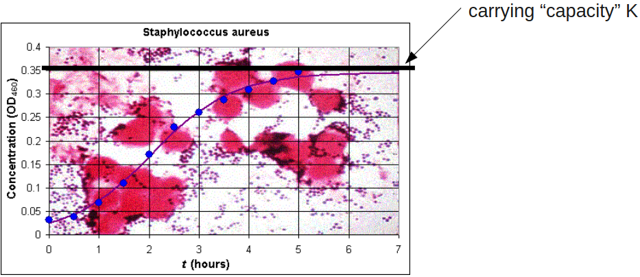
Initially, we would think to plot this as some model of exponential growth, which has a differential equation of the form:
We can then introduce the notion of this capacity \(k\), with a constraint on the space or the available food to reduce the growth rate. The first idea introduced here is that we decrease the growth rate linearly with \(P\):
This equation could be solved, or we can look at the equilibrium states, i.e., when the gradient of the equation is zero:
Here, we see that we have two solutions for the equation: \(P^{stat} = 0\) or \(P^{stat} = k\). Therefore, we can see, in the long run, where the system will end up (at either of these static points).
Stability
Stability in the system can differ based on the initial conditions of the system. The example shown showed that we had two possible stable states, at \(P^{stat} = 0\) and at \(P^{stat} = k\).
We can analyse which state the system will end up in by using phase portraits, which we'll cover momentarily. We can also look at the stability of the stationary states.
In the lecture notes, they define a state as being stable if the system relaxed back into the state after some perturbation, and unstable otherwise. This is shown with the following phase portrait:

We can then test this by numerically integrating with some sample trajectories at \(P(0) = 0,100, 1000, 2000, 2500\).

We see that for all values of \(P(0) \ne 0\), they eventually converge at \(2000\), with the \(P(0) = 0\) remaining at zero.
Non-Linear Example
We have so far seen in terms of a linear equation that can be solved analytically. If we now consider \(\frac{dx}{dt} = \sin(x)\) and plot for different values of \(x\) on the \(x\)-axis, we see that there are 5 roots in \([-2\pi, 2\pi ]\). These occur at \(-2\pi, \pi, 0 \pi, 2\pi\). Technically, this equation is linearly separable, so can be solved analytically, but is still non-linear.
Of these points, the points at \(-\pi\) and \(\pi\) are stable, with the remainder being unstable, as shown by the solid circles and the hollow circles.
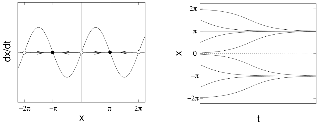
If we then plot the values of \(x\) against \(t\), where \(t\) is on the \(x\)-axis, we see that for all values even close to the unstable fixed points, we eventually converge on one of the stable points.
We can see the stability of this, because whenever the line is above the \(x\)-axis, we are moving right, and whenever it is below the \(x\)-axis, then we are moving left.
Quantifying Fixed Points and Stability Analytically
So far, we have looked at how we can find fixed points by looking at graphs of the \(\frac{dx}{dt}\) against \(x\) and then the plots of a numerical solution to \(x\) and \(t\). We can now look at how we might approach these solutions analytically.
For a general system, with some differential equation \(\frac{dx}{dt} = f(x)\), we can imagine a fluid that flows along the real line with a local velocity \(\frac{dx}{dt}\). We can then mathematically define when a solution is a fixed point:
We have also discussed the notions of stability, with small perturbations dampening out in the long term being classified as stable, and small perturbations that grow in the long term being classified as unstable.
Example: \(\frac{dx}{dt} = x^2 - 1 = f(x)\)
For this, we want to initially classify the dynamics by analysis of the fixed points. We set the equation equal to zero, then factorize to get the roots:

From these roots, we can see that \(x_1\) is unstable, and \(x_2\) is locally stable, but not globally stable. Some perturbation may be enough to destabilize \(x_2\). Again, this has been shown geometrically, and we have been reasoning about the stability based on the graph we see.
Quantifying Perturbations
Take a fixed point \(x^* = x^{stat} | f(x^*) = 0\), then we can consider the fate of a small perturbation \(\epsilon = x(t) - x^*\) from this.
As \(\frac{dx}{dt}(x^*) = 0\), we can insert it into a differential equation for \(\frac{d\epsilon}{dt}\), which will yield \(\frac{dx}{dt} = f(x + \epsilon)\).
We can then expand this \(f(x+\epsilon)\) in a Taylor series around the point \(x^*\):
As we are only interested in the size of the perturbation from the original function, we can eliminate the \(f(x)\) from the RHS of the function, yielding:
Now, from this equation, we can see that the perturbation will grow exponentially if the gradient \(\frac{df}{dx} > 0\), will decline exponentially if \(\frac{df}{dx} < 0\), and if \(\frac{df}{dx} = 0\), then we have marginal stability, and we need to expand into higher orders to see what is going on.
To look at how quickly the system returns to the equilibrium, we can look at the gradient we get, and we will return with a characteristic timescale \(1/ | \frac{df}{dx} |\). The larger this value is when evaluated at \(x^*\), the quicker we return to the equilibrium point.
Algebraic Solution to Logistic Growth
If we now return to the earlier example of \(\frac{dP}{dt} = rP(1-\frac{P}{K} = f(P)\), knowing the two fixed points at \(P^{stat} = P^* = 0,K\), we can linearize the equation around these points.
At \(P=0\), we yield \(f(0+\epsilon) \approx r \epsilon\)
At \(P=K\), then we yield $f(K+\epsilon) \approx f
Unfinished bit here, don't fully understand
Example: \(\frac{dx}{dt} = \sin x\)
For \(f(x) = \sin x\), we have fixed points at \(f(x) = 0\) and \(x = k \pi \forall k \in \mathbb{Z}\).
The stability of this can be categorized by taking \(\frac{df}{dx} = \cos x = \cos k \pi\). Where this is above 0, the fixed point is unstable, and if negative, then we converge back to the fixed point.
From this, we can see that \(\forall k\) that are odd, the stability is stable, and for all even \(k\), the stability is unstable. (Wow Charlie can you write a more stupid sounding sentence?)
Handling \(\frac{df}{dx}=0\)
In this instance, we have a number of different things that can happen, based on the underlying function. Take a look at the following examples, and you'll see that the stability is dependent on what the function does after the fixed point:

Extending Beyond 1D
So far, we have all functions in one dimension. With these functions, they either tend to a fixed point in the long term, or to \(\pm \infty\). These are the only possible dynamics that we can see from a 1D system.
This is because a 1D system has a flow along the real line. If the flow is monotonic on this line, then we will never come back to a starting position. If we now consider higher dimensions, such as 2D or more, then we can have similar behaviour to what was seen in earlier lectures.
We will either get linear oscillations, limit cycles, or chaos.
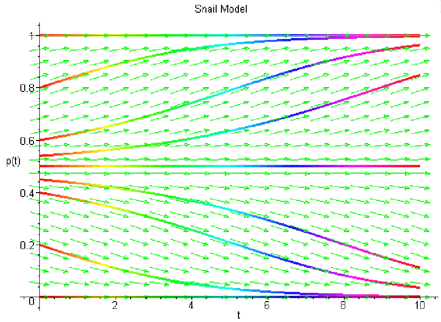
Example: Sinistral and Dextral Snails
Given two snails with opposing shell winding directions, we want to have the ability to characterise what will happen to a population with different ratios of Dextral and Sinistral snails, at least in theory.
Assumptions: likelihood of a sinistral breeding with dextral is \(\propto\) the product of their numbers; breeding like with like produces their own type; breeding different pairs gives both types with equal probability.
We can then start to think of the equation for this. If the likelihood that a randomly picked snail is sinistral is given by \(p\), then the temporal dynamics of this is given by:
We can derive stationary points where \(f(p^{stat}) = 0\), by solving the equation for \(p\). We have three roots, \(0,1,\frac{1}{2}\). Let's examine the stability of this equation and the roots. We can do this visually, with the \(\frac{dp}{dt}\) on the \(y\)-axis and the \(p\) on the \(x\)-axis.

We can also numerically integrate, to see where we end up in the long term:
Analytically, we can first take the derivative, which is easier done if we first expand out the equation:
Now, we can feed in the fixed points, giving us the stability of each:
This shows that there can be no coexistence of these species of snail.
Quick Jot Notes
These notes were what I took on the first pass of the lecture, before I came back and rewatched it taking my actual notes.
- Sometimes we have nonlinear systems of equations
- Might not want to solve them properly
- Instead of solving, we can plot the \(dx/dt\) on the \(y\)-axis and the time on the \(x\)-axis, This then shows zero-crossings
- Each zero-crossing is a stationary point, then can look at direction of travel for flow
- Can compare with numerical integration results for different starting conditions to see emergent behaviour (\(x\) on the \(y\)-axis and \(t\) on the \(x\)-axis)
- Stable full dots on line
- Hollow dots are unstable equilibria
- Small perturbations -> local stability
- Any perturbation -> global stability