Palm Biometrics

Paper Notes

Full paper notes I took in the session are available here in case they don't make sense in the context of the text as inserted.

Palm biometrics are one of the oldest biometrics systems in use. The handprint from one individual varies to that of another, and as early as 1858, this type of biometric has been used to verify the authenticity of a contract. In 1973 came the use of the identimat, the first commercial hand reader.

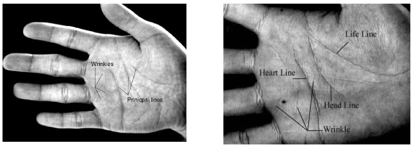
The palm has many features which vary from person to person. These include the wrinkles in the skin, and the three principal lines: the heart line, the head line, and the life line. A paper giving a technique on how to do this is D. Zhang, W-K. Wong et. al, IEEE TPAMI, 25 2003.

Method of Recognition

To detect a person by their palm, they place their palm in a machine with a camera and a light source to light the palm. This camera then feeds the picture into the computer, which then goes into the processing pipeline.

Preprocessing

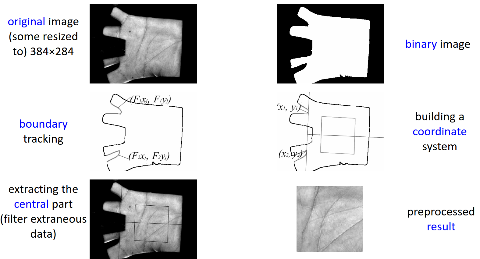
The original image may be resized to some smaller dimension (e.g., 384x284 pixels). We can then take a binary mask of the image, so that we have only the palm in our processing algorithm. We can then do boundary tracking of the palm, and build a coordinate system around the location of the fingers relative to the palm. We take the line between two points, then the normal to that line about its centre point, which gives the centre of the coordinate system.

From this coordinate system, we can extract the central part of the palm, filtering any extraneous data. The masking can help prevent extraction of features from the background or unwanted regions, and can be used in the case the palm was not placed correctly in the image.

Principal Lines

These cannot be used for recognition, as multiple people can have very similar principal lines on their hands. Therefore, we may look to get the wrinkles in the hands as our feature to extract and compare.

Gabor Wavelets

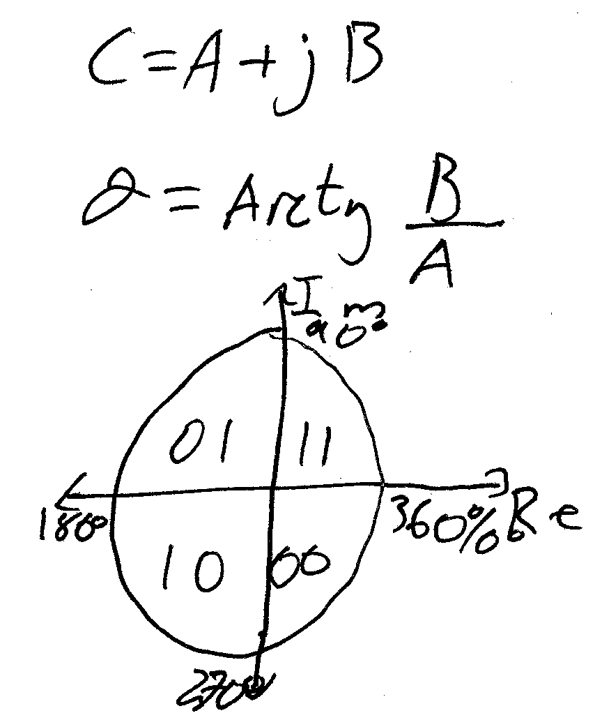
Once again, old trusty makes an appearance. We filter the preprocessed images with a bank of Gabor wavelets, then similar to iris recognition techniques, we extract two binary bits for the phase of each of the wavelet outputs, then look at the corresponding masks we get, and their similarity to data already stored.

Recall that this is Daugman's method in use.

Matching

We take the normalised hamming distance between the real \(\Re\), imaginary \(\Im\), and mask \(M\) of the images:

Equation not covered in the lecture

Sasoon very briefly discussed this as the Hamming distance, but did not discuss the constituent parts of the equation. Therefore, probably need to refer to its usage in the Iris Biometrics lectures.

\[ D_0 = \frac{ \sum_{i=1}^N \sum_{j=1}^N P_M(i,j) \cap Q_M(i,j) \cap (P_{\Re}(i,j) \otimes_{\Re}(i,j)) + P_M(i,j) \cap Q_M(i,j) \cap(P_{\Im}(i,j) \otimes Q_{\Im}(i,j)) }{ 2\sum_{i=1}^N \sum_{j=1}^N P_M(i,j) \cap Q_M(i,j) } \]

The hamming distance is then bounded \(<1\), and the lower the distance is the better the match. Here, \(\otimes\) is equal to zero if the two bits are the same. The histogram for this is normalized.

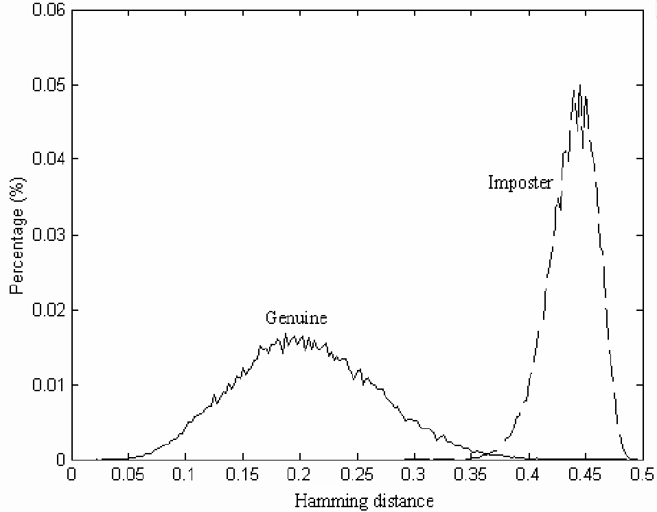
Again, the binary output follows a binomial distribution. For a genuine print, there is a distribution around the 0.2 mark, with a spread from 0.05 to approx 0.4, with imposter prints at around the 0.45 mark.

ROC Curve

The ROC curve, as plotted between the genuine acceptance rate and the false acceptance rate gives an EER of 0.6%, which is comparable to other palm print recognition approaches.

Time Variance

As with all biometrics, we want them to be invariant to the ageing of the person. We can plot the hamming distances of each image compared with the other images, at a difference in time, which yields the following table for the images \((a),(c),(e)\) as the first collected images, and \((b),(d),(f)\) as the second collected images with a mean time of 69 days, a minimum of 4 days and a maximum of 162 days between prints.

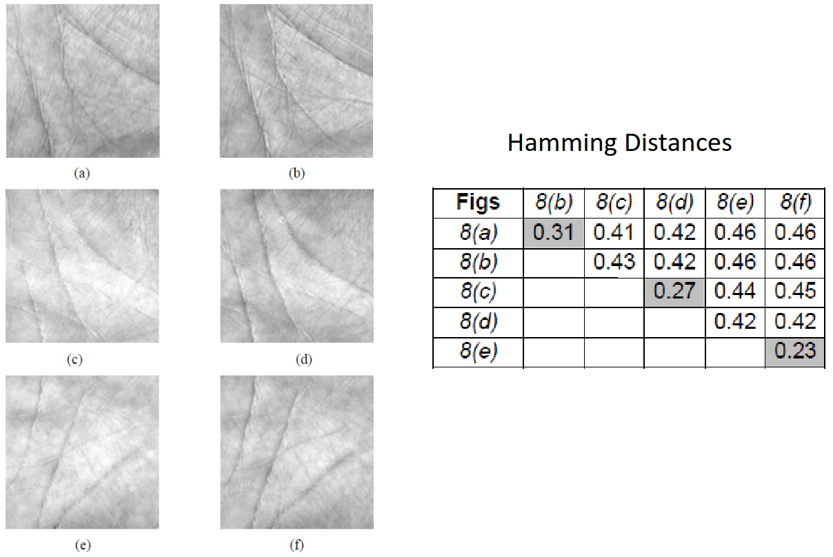
The hamming distances remain small between the same person to a quantifiable amount.

Illumination

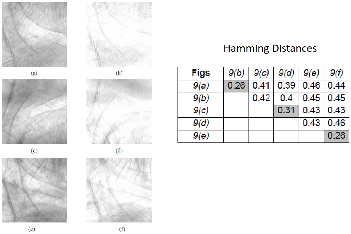
Similarly, we can study the effects of illumination on the hands to see how a brighter or darker picture may be perceived by this bank of Gabor filters. Again, the hamming distances for different lighting levels of the same individuals \((a),(c),(e)\) as reference, and \((b),(d),(f)\) as the adjusted level, we can still noticeably isolate the same individuals within the table.

Eigenpalms (PCA)

This is a method that uses PCA given a dataset of palms. With the dataset, they can produce the eigenvectors and eigenvalues from the dataset, in a similar way to how they were produced for face recognition. This was proposed by Lu, Zhang et al. Pattern Recognition Letters 24, 2004.

First of all, we take an image of values \(I\), and linearize it into an \(N^2 \times 1\) vector of all components within the image:

Here, the generated vector is denoted \(\vec{v}\). We do this for all images in the entire dataset \(\vec{v_1},\vec{v_2},\dots,\vec{v_n}\), then generate an average, or mean, vector:

\[ \vec{v_m} = \frac{1}{m} \sum \vec{v_i} \]

We can then use this to generate a covariance matrix of size \(N\times N\):

\[ C_{(N \times N)} = \frac{1}{m} \sum (v_i - v_m)_{(N \times 1)} (v_i - v_m)_{(1 \times N)}^T \]

Here, the subscript brackets denote the size of the respective matrices. With the covariance vector, we can try to solve the following equation for \(\vec{x} \ne 0\):

\[ \underbrace{(C - \lambda I)}_{\text{must be singular, i.e. }\det = 0} \vec{x} = 0 \]

Here, \(I\) is simply the \(N \times N\) identity matrix. We can then use \(|\vec{x}| = 1\) to compute the \(e_i\)s for the matrix, for \(\lambda_1,\lambda_2,\dots,\lambda_N\).

We then yield eigenvectors \(\vec{e}\), with eigenvalues \(\lambda\). We can arrange these eigenvectors back into an image as we had initially, by decomposing the \(N^2 \times 1\) matrix into a matrix of \(N \times N\). This yields the pictures that we see for the eigenpalms, and in the case of face recognition, the various features we extract from the face.

As these eigenvectors and eigenvalues are linear, any linear combination of these can create our vector

\[ \vec{v}_i = a_1\vec{e_1} + a_2 \vec{e}_2 + \cdots + a_n \vec{e}_n \]

We can use a limited number of eigenvectors, ignoring those vectors with small eigenvalues. If we reduce the number of dimensions of the feature vector \(A\), then we might yield a higher accuracy.

The paper claims an accuracy of 99.149% based on their 91 features used.

These eigenpalms can be seen below:

By Shape and Texture

This allows us to do the classification by the features from an image. Another way to do this is by the shape and texture of the hand itself. This was introduces by A. Kumar, D. Zhang et. al, IEEE TIP 24, 2005.

We can make use of lots of different measurements from the hand, e.g., finger length, palm length, perimeter of hand, finger width, overall length. Another way is through the use of a silhouette of the hand. This was introduced by Kumar et al, Pattern Recognition Letters 27, 2006.

Extraction of Two Palm Biometric Modalities

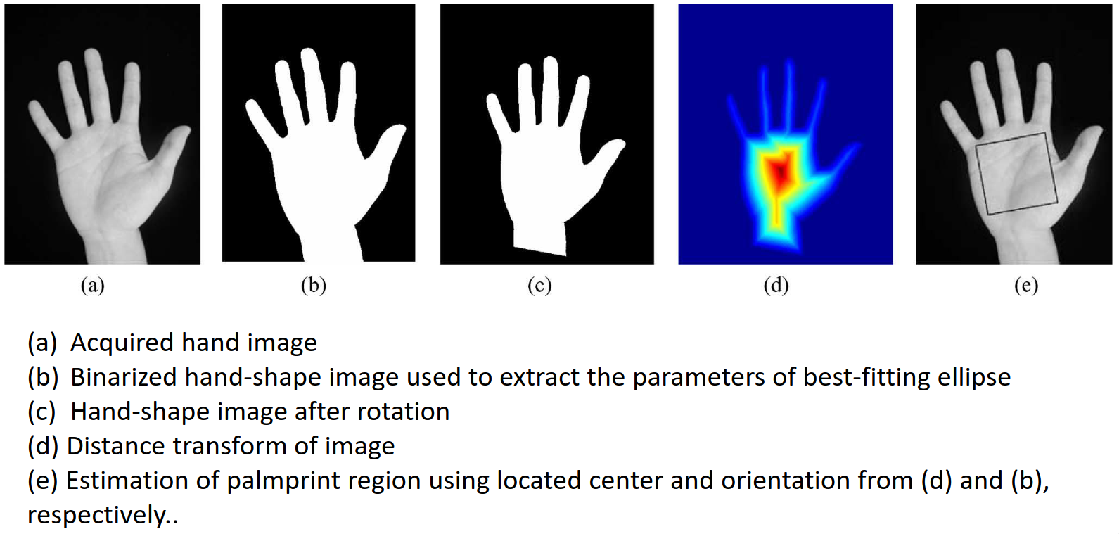
We first have the image of the hand, which we then binarize and extract parameters of a best fitting ellipse. This best fitting ellipse comes from the edges of the best fitting silhouette. Be prepared for the world's worst drawing of a hand drum roll please:

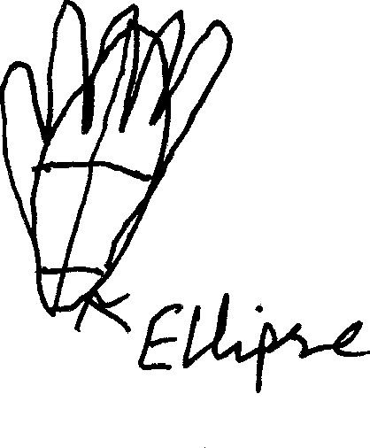
The ellipse may not be vertical in the original image. We then rotate this ellipse to get the hand vertical.

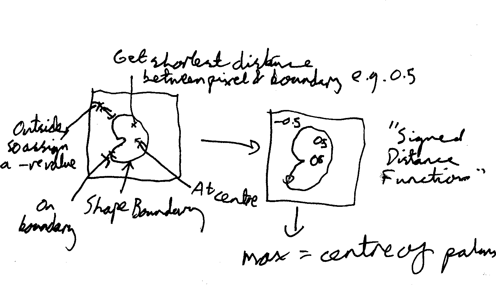
We can then get a region of interest which surrounds the maximum point of the distance function. This gets us the distance transform of the image, and we can the define the estimate of the palmprint region using the centre and orientation of the main image. This corresponds to the heatmap seen in part \((d)\) of the image above.

The heatmap can be extracted by taking the transform, running some form of edge detection on the edge map, then taking the distance from each of the pixels to the nearest edge in the edge map. We then plot the values of the distances, using a negative value where the point is outside the hand (dark blue on the image), and a positive value inside the hand. Pixels on the edge will have a value of zero.

The maximum distance from the edge as plotted will be the centre of the palm, given our algorithm.

We can now combine the image extraction techniques by segmenting, then fitting an ellipse, rotating, finding the centre of the silhouette, then substituting the greyscale version of the hand back in, which then allows us to plot the location of the palmprint.

Processing of Palmprint

Now we have the segmented image, we can apply the usual preprocessing techniques to normalize it:

Then taking directional masks at 0°, 90°, 45°, and 135°:

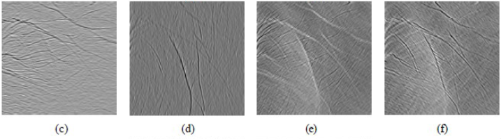
We then combine these four images into \((g)\) below, then extract features from each overlapping block:

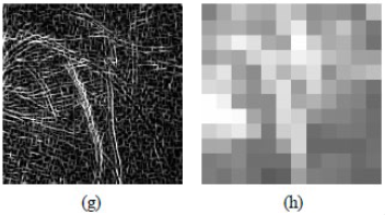
To yield \((g)\), we take the maximum value from each of \((c,d,e,f)\), then the features are standard deviations of these blocks.

Performance with Fusion

We have now looked at two different methods we can use to quantify a palmprint. The first is to do with the overall shape of the hand, known as hand geometry, and the latter is the palmprint. Distance \(s = \frac{v_pv_q}{|v_p||v_q|}\) is the cosine distance:

\[ v_p v_q = |v_p||v_q| cos \theta_{pq} \]

and plot a graph of the distribution of genuine and imposter scores for palmprints, with the palmprint on the \(y\)-axis, and the hand geometry on the \(x\)-axis, and also plot 3 series (individual, combination of both techniques) on a ROC curve, to see which performs better:

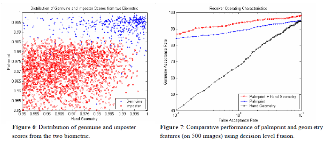
From the plot on the left, we can see that the genuine prints and imposter prints seem to segment themselves nicely, with the scores of genuine mostly being at the higher end of the spectrum, and the scores of the impostors being lower on both metrics.

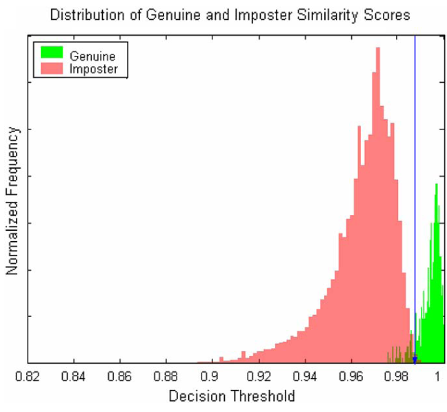
From the ROC curve, we can see that the combination of both metrics is the best, with the print being a much better measure than the shape of the hand. We can then further plot a histogram of the similarity scores on a normalised plot, where we see that the decision threshold can be put nicely between the two peaks:

Partial Model Based Approach

This was another approach proposed by J. You et al., Pattern Recognition, 35, 2002, which splits the palmprint into several regions based on the locations of the principal lines and the datum points. Here, we have three regions: \(I\) is the finger-foot region, \(II\) is the inside region, and \(III\) is the outside region. Line \(1\) is the heart line, \(2\) is the head line, and \(3\) is the life line. We have datum points \(a,b\) which are the endpoints and \(o\) which is the midpoint of \(ab\).

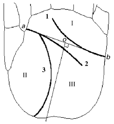
These features can be extracted if we print palmprints on paper by inking a palm, then placing it on the paper. These paper prints can then be digitised. These scans will reveal the principal lines, wrinkles, and ridges of the palms

Texture Features

Palmprints can have varying features that categorise them. These include strong principal lines, number of wrinkles, and the strength of the wrinkles. We can use these similarities to aid with classification, but many people have lots of wrinkles, or strong principal lines.

Laws' Filters

These are filters that we convolve with palm images, and are zero-sum, or high pass, filters. A sample of 5x5 filters can be seen below.

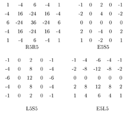
After application of these filters, we can extract the mean, variance, mean deviation etc., which we can then use as features for classification.

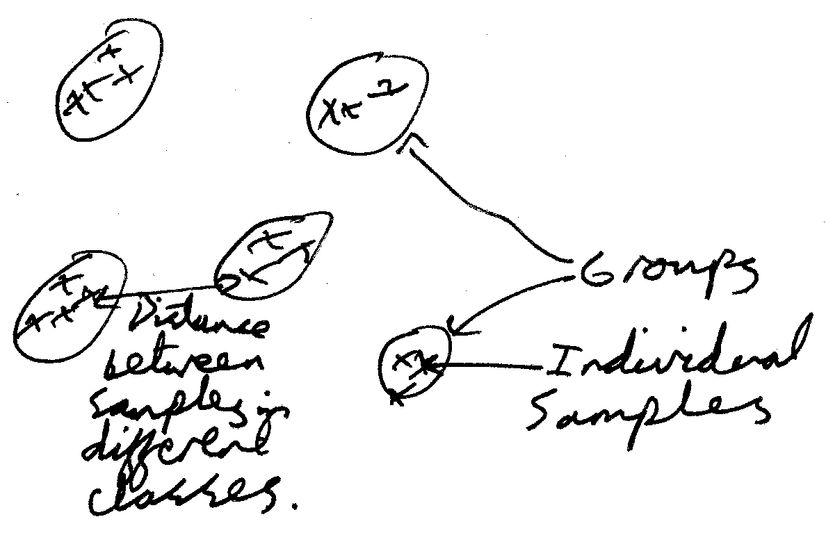
Feature Point Detection for Matching

We can also extract interesting points from palm scans, if we run edge detection, then extract corners, terminated points, and points on rings and spirals.

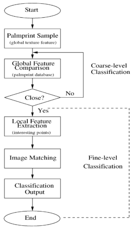
Classifier

The classifier for this particular paper looks as follows:

Congratulations, [insert name here]! You've reached the end of my biometrics notes.