Numerical Methods for Integration and Differentiation

All the content we have covered so far examines the difference between analytical methods, i.e., those that provide exact solutions, and numerical methods, which are those that provide approximations, which we can iterate over to get a solution that is correct up to a specified error boundary.

As discussed in the modelling and modelling cycle lecture, different disciplines often value different aspects of their models. Physicists, for example, will usually like a solution that is numerically very accurate and close in value to the theoretical value.

Taylor Series

One concept that has already appeared but hasn't been formally discussed is the Taylor series. This is an important concept that is used in many different algorithms. If we have a smooth function \(f(x)\), we can compute the Taylor series of that function around a specific point \(c\).

The Taylor series will often rapidly converge around the point \(c\), but diverge if it is far away from \(c\). The general formula of the series is:

\[ f(x) \approx f(c) + \frac {f'(c)}{1!}(x-c) + \frac{f''(c)}{2!} (x-c)^2+\frac{f'''(c)}{3!}(x-c)^3+ \cdots = \sum_{n=0} ^ {\infty} \frac {f^{(n)}(c)}{n!} (x-c)^{n} \]

Convergence

We need to know what the error of the function is. The definition for the series above continues to approximate to the \(\infty\)-th polynomial. When actually using the Taylor series in practice, we have to bound the degree of this polynomial, and we can also see that the amount the \(n\)-th degree polynomial factors in is proportional to \(n!\).

In practice the error term at \(E_{n+1}\) approximates the \(n+1\)-th polynomial, as this will be the largest value of the terms that aren't used:

\[ \begin{align} E_{n+1} &= f(x) - f_n(x)\\ &= \sum_{k=n+1}^\infty \frac{f^{(k)}(c)(x-c)^k}{k!} \\ &\approx \frac{f^{(n+1)}(\zeta)(x-c)^{n+1}}{(n+1)!}\\ \text{where } \zeta &\in [x,c] \end{align} \]

Familiar Examples

There are Taylor approximations to many continuous functions, such that the definitions become something that is easier for a computer to calculate. The following are all good examples of where the Taylor approximations of functions are used:

\[ \begin{align} e^{x} &= \sum^{\infty}_{n=0} \frac{x^n}{n!} = 1 + x + \frac{x^2}{2!} + \frac{x^3}{3!} + \cdots\\ \sin x &= \sum^{\infty}_{n=0} \frac{(-1)^n}{(2n+1)!} x^{2n+1} = x - \frac{x^3}{3!} + \frac{x^5}{5!} - \cdots && \text{for all } x\\ \cos x &= \sum^{\infty}_{n=0} \frac{(-1)^n}{(2n)!} x^{2n} = 1 - \frac{x^2}{2!} + \frac{x^4}{4!} - \cdots && \text{for all } x\\ \frac{1}{1-x} &= \sum^\infty_{n=0} x^n = 1 + x + x^2 + x^3 + \cdots\\ \end{align} \]

For a computer to calculate a value to a certain number of digits of accuracy, we simply sum over the terms, until the \(n\)th term will not change the first \(m\) digits of the output.

For the calculation of \(e\), for example, we would use the Taylor expansion up to the ~9th term:

\[ e = e^1 = 1 + 1 + \frac{1}{2!} + \frac{1}{3!} + \frac{1}{4!} + \frac{1}{5!} + \frac{1}{6!} + \frac{1}{7!} + \frac{1}{8!} + \frac{1}{9!} \]

The \(\frac{1}{9!}\) term gives \(2.76\times10^{-6}\), so the output is correct to \(10^{-5}\). In practice, most compilers will have the value for \(e\) precomputed, e.g., Go.

Numerical Differentiation

We want to be able to approximate the derivative of functions \(f(x)\) and higher orders of differentiation. We can recall from the differentiation by first principles the simple formula:

\[ f'(x) = \lim_{h \to 0} \frac{f(x+h) - f(x)}{h} \]

Mean Value Theorem

Using Taylor's theorem, we can set \(n=0\), and derive the mean value theorem. This is a theorem that states for an arc between two points, there is at least one point on that arc which is parallel to the secant through its endpoints. This is best illustrated with the graph from Wikipedia (CC BY-SA 3.0, author 4C):

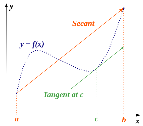
The lecture slides show a very primitive derivation of this:

\[ \begin{align} f(x) - f(b) &= (b-a)f'(\xi)\\ f'(\xi) &= \frac{f(b) - f(a)}{b-a} \end{align} \]

The main takeaway here is that we can use this to approximate \(f'\) if the interval \((a,b)\) is small.

Finite Difference Schemes

This is really quite simple. We use the differentiation from first principles idea, but then slightly alter the formula depending on what we want to work on. There are 3 main finite difference schemes:

\[ \begin{align} \text{Forward Difference:} \quad f'(x) &\approx \frac{1}{h}(f(x+h)-f(x))\\ \text{Central Difference:} \quad f'(x) &\approx \frac{1}{2h}(f(x+h)-f(x-h))\\ \text{Backward Difference:} \quad f'(x) &\approx \frac{1}{h}(f(x)-f(x-h)) \end{align} \]

These schemes will have slight errors, known as truncation errors. This is because the functions are expanded into a Taylor series of some order and neglecting certain orders of this series.

Taking, for example, the central difference from the finite difference schemes, we see that the Taylor series of this would be:

\[ \begin{align} f(x+h) &= f(x) + hf'(x) + \frac{1}{2}h^2f''(x) + \frac{1}{6} h^3f'''(x) +O(h^4)\\ f(x-h) &= f(x) - hf'(x) + \frac{1}{2}h^2f''(x) - \frac{1}{6} h^3f'''(x) +O(h^4)\\ \text{If we then rearrange to get into difference:}\\ f(x+h)-f(x) &= hf'(x) + \frac{1}{2}h^2f''(x)+\cdots\\ \frac{1}{h} (f(x+h)-f(x)) &= f'(x) + \underbrace{\textcolor{red}{\frac{1}{2}hf''(x)+\cdots}}_{\text{Error is }1^{\text{st}} \text{ order in }h}\\ \text{And for the backward difference:}\\ \frac{1}{h} (f(x)-f(x-h)) &= f'(x) - \underbrace{\textcolor{red}{\frac{1}{2}hf''(x)+\cdots}}_{\text{Error is }1^{\text{st}} \text{ order in }h}\\ \text{But central difference:}\\ \frac{1}{2h}(f(x+h) - f(x-h)) &= f'(x) + \underbrace{\textcolor{blue}{\frac{1}{6}h^2f'''(x) + \cdots}}_{\text{Error is }2^{\text{nd}} \text{ order in }h}\\ \end{align} \]

Here the \(O\) means the order of the function, which will be quartic. \(h\) should be very small in value. As highlighted in red, the approximation of the function at both the forward and backward difference is 'first order in \(h\)', meaning that the error is proportional to the size of \(h\).

The blue equation gives the error in the second order of \(h\), so as the size of \(h\) decreases, the error decreases exponentially in terms of \(h^2\). To derive the central difference, we take the first equation in terms of the Taylor expansion, then subtract the second. These terms then mostly cancel out.

The key takeaway from all this is that the central difference scheme is the best, as it has a lower error than the forward and backwards schemes.

Higher Order Derivatives

This is all good and well for taking the first derivative, but we'd also like to calculate second, third, etc. derivatives too. We could naïvely do this using the central difference from the first derivative, but this has downsides in that we are then compounding errors, and have to do many different calculations.

If we instead take the Taylor expansions \(f_4(x+h)\) and \(f_4(x-h)\) (here \(_4\) just means that it is the Taylor expansion to the fourth degree), then we can sum them together, and we will see that we are left with \(f''(x)\) as the first term that doesn't cancel out. Derivation.

To obtain a higher order accuracy than the 2nd order, we can write the Taylor expansions of \(f(x+h), f(x-h), f(x+2h), f(x-2h)\). Then we can combine these to eliminate truncation error terms.

This does, however, mean that we have to run the function \(f(x)\) for more iterations, which can be quite costly depending on the model. We determine the truncation errors as a part of our models, as whilst computers can work on small values of \(h\), they typically have issues storing these accurately, and the small errors in each iteration can quickly compound.

The general idea behind the finite calculation errors is that the error is simply the difference between the full Taylor expansion to the infinite degree, and the order of the method that we are using.

Multivariate Taylor

Later in this module, we will be using functions \(f(x,y,z,\dots)\), which we would like to have the ability to represent as a Taylor series.

To make this nice, we introduce multi-indices:

\[ \alpha \in N^n, \alpha = (\alpha_1, \dots, \alpha^n), |\alpha| = \sum_{j=1}^n \alpha_j \]

Then, for the factorial term, we have:

\[ \alpha! = \alpha_1 ! \cdot \alpha_2 ! \cdot \dots \cdot \alpha_n ! \]

We can then introduce the notion of \(\vec{x^\alpha}\):

\[ \vec{x^\alpha} = x_1^{\alpha_1} \cdot x_2^{\alpha_2} \cdot \dots \cdot x_n^{\alpha_n} \]

And then the partial derivative matrix of \(\alpha\) with respect to \(f\):

\[ D^\alpha f = \frac{\delta^{|\alpha|}f}{\delta x_1^{\alpha_1} \delta x_2^{\alpha_2} \cdots \delta x_n^{\alpha n}} \]

We can then compute \(f(\vec{x} + \vec{h})\):

\[ f(\vec{x} + \vec{h}) = \lim_{k \to \infty} \sum_{|\alpha| \le k} \frac{1}{|\alpha|!} D^\alpha f(\vec{x})\vec{h^\alpha} \]

Breaking this down, we have the \(\sum_{|a| \le k}\) term, which essentially says that the order is less than or equal to the order we want to expand for that Taylor expansion.

The \(\frac{1}{|\alpha|!}\) term is the factorial of the order for that part, so when \(\alpha=0\), then we have \(\frac{1}{0!} \stackrel{\triangle}{=} 1\). Then we have the \(D^\alpha f\), which is the partial derivative matrix, then we multiply through by a \(h\), specific to each \(\alpha\), and increasing in power.

Then, we expand \(f(x,y)\) to a specific order. Here, the second order makes sense as anything higher is just tedious to write out.

\[ \begin{align} f(x+h_1, y+h_2) &\approx f(x,y) &&\text{(linear term, }\alpha=0\text{)}\\ &+ \delta_xfh_1 + \delta_yfh_2 &&(\alpha=1)\\ &+ \frac{1}{2!} \delta_x^2fh_1^2+\delta_x\delta_y h_1 h_2 + \frac{1}{2!} \delta_y^2h_2^2 \end{align} \]

Clarity Following Problem Sheet

This was confusing until I finished question 2 of the problem sheet. Essentially, when we expand a Taylor series around a point in a linear function, we have a single term for constant, \(x\), \(x^2\), \(x^3\). In multivariate Taylor, for the first order, we have a term for \(x\), and a term for \(y\) (in the instance of two variables), or \(x\), \(y\), \(z\) in the case of three variables.

For the next part, we start to combine those variables in different ways, so we'd have \(x^2, y^2, xy, yx\) for the second bit. Each of these is then combined with the partial derivative \(\frac{df}{dx^2}, \frac{df}{dy^2}, \dots\).

For calculating the partial derivatives, I found it useful to make use of a Hessian matrix, which combines each of the combinations of the second partial derivatives, then we can simply plug in the value at \(a\) to these partial derivatives and have the Taylor expansion.

Numerical Integration

Given \(f(x)\) in \([a,b]\), we want to find an approximation for the integral of \(f\):

\[ I(f) = \int_a^b f(x) dx \]

The main strategy for this is to cut \([a,b]\) into some sub intervals, then at each interval \(i\), approximate \(f(x)\) with a polynomial equation \(p_i\). We can then integrate the individual polynomials analytically at each interval then sum their contributions.

Initially, we could approximate \(f\) by a constant at each sub-interval, so \(p_i(x) = f(x_i) = f_i\) for that entire interval. This has issues in that the small almost triangle parts are left out.

For this, we get each integrand as:

\[ \int_{x_i}^{x_{i+1}} p_i(x)dx = \int_{x_i}^{x_{i+1}} f_idx = f_i(x_{i+1}-x_i) \]

So, if we have equidistant intervals, the overall form would be:

\[ \int_a^b f(x) dx \approx \sum_{i=0}^{n-1}f_i(x_{i+1}-x_i) \]

We know that the step is \(h = \frac{b-a}{n}\), and \(x_i = x_0 + (i-1)h\). Therefore we can approximate \(\int_a^b f(x) dx \approx h \sum_{i=0}^{n-1}f_i\).

Trapezoid Rule

This is similar to above, but instead of using rectangles, we use trapezoids, using a linear polynomial that connects both the points it intercepts.

We know that on any given interval \([x_i, x_{i+1}]\), we can interpolate \(f(x)\) by a linear polynomial, such that \(f(x_i)=p_i(x_i)\), and \(f(x_{i+1}) = p_i(x_{i+1})\).

We can do this using the straight line formula \(y-y_1 = \frac{(y_2 - y_1)}{(x_2 - x_1)} (x-x_1)\):

\[ p_i(x) = f(x_i) + (x-x_i) \frac{f(x_{i+1}) - f(x_i)}{x_{i+1} - x_i} \]

To get the area of this, we can integrate the above function, which would give:

\[ \begin{align} \int_{x_i}^{x_{i+1}} p_i(x)dx &= \left[ f(x_i) x - x_i x \frac{f(x_{i+1}) -f(x_i)}{x_{i+1} - x_i} + \frac{x^2}{2} \frac{f(x_{i+1}) - f(x_i)}{x_{i+1} - x_i} \right]_{x_i}^{x_{i+1}}\\ &= \frac{1}{2}(f(x_{i+1}) + f(x_i))(x_{i+1}-x_i) \end{align} \]

This gives the general form for the area of a trapezium. Similar to the constant approximation at each interval, we can sum over all the intervals:

\[ \begin{align*} \int_a^b f(x) \, dx &\approx \sum_{i=0}^{n-1} \frac{1}{2} \left( f(x_{i+1}) + f(x_i) \right) (x_{i+1} - x_i)\\ h &= \frac{b-a}{n}, \quad x_i = x_0 + (i-1)h\\ \int_a^b f(x) \, dx &\approx \sum_{i=0}^{n-1} \frac{h}{2} \left( f(x_{i+1}) + f(x_i) \right) \\ \int_a^b f(x) \, dx &\approx h \left[ \frac{1}{2} f(x_0) + \sum_{i=1}^{n-1} f(x_i) + \frac{1}{2} f(x_n) \right] := T(f; h)\\ \end{align*} \]

This gives an estimate, given a function \(f\) and a step \(h\) as parameters. The error to this function is \(E(f;h) = I(f) - T(f;h)\), where \(I\) is the actual integral, and \(T\) is the approximation. The error in the integral is therefore:

\[ \sum_{i=0}^{x_{i+1}} [ f(x) - p_i(x)] = \sum_{i=0}^{n-1} E_i(f;h) \]

Approximating the function linearly at each interval yields an area \(\propto h^2\). The integration of these errors yields an error order \(E_i \propto h^3\), then the summation of all these \(h\) different splits of the function again brings us an error \(E \propto h^2\).

Simpson's Rule

Current approximations show that if we approximate by a constant for interval \(h\), then the error is \(\approx h\). If we approximate with a linear function, then \(E \approx h^2\). For a quadratic function, we apply Simpson's rule.

The lecture slides delve no further than to introduce it and show that for an integral \(I\), \(S(f;h)\) is the Simpson's rule approximation, giving:

\[ I \approx S(f;h) = \frac{h}{3} \sum_{i=0}^{n-1} [f(x_{2i} + 4f(x_{2i+1} + f(x_{2i+2})] \]

We can then show that Simpson's rule is 4th order, \(E \propto h^4\).

Recursive Trapezoid

All the methods so far approximate using a specified number of computations, regardless of how much or little the approximation error is affected at each stage. The recursive trapezoid method controls truncation error without making too many unnecessary computations. It starts by dividing the interval \([a,b]\) into \(2^n\) sub intervals, then evaluates the trapezoid rule for \(h_n = 2^{-n}(b-a)\) and \(h_{n+1} = \frac{h_n}{2}\)

This approach has advantages in that the computations can be kept at a specified level \(n\). If that is not accurate enough for us, then we can add another level. We also don't need to re-evaluate points that have already been evaluated at a previous level.

\[ \begin{align*} \text{For } h_{n}\colon \quad T(f; h_n) &= h_n \left[ \frac{f(a) + f(b)}{2} + \sum_{i=1}^{2^n-1} f(a + ih_n) \right] \\ \text{For } h_{n+1}\colon \quad T(f; h_{n+1}) &= h_{n+1} \left[ \frac{f(a) + f(b)}{2} + \sum_{i=1}^{2^{n+1}-1} f(a + ih_{n+1}) \right] \\ \text{We can show:} \quad T(f; h_{n+1}) &= \frac{1}{2} T(f; h_n) + h_{n+1} \sum_{j=0}^{2^n-1} f \left( a + (2j+1)h_{n+1} \right) \end{align*} \]

Romberg Method

This is another method we can use to get a good approximation. If we have \(T(f;h), T(f;h/2), T(f;h/4)\), we can show that:

\[ \begin{align} E(f;h) &= I(f) - T(f;h) \\ &= a_2h^2 + a_4h^4 + a_6h^6+\dots\\ E(f;h/2) &= I(f) - T(f;h/2)\\ &= a_2(h/2)^2 + a_4(h/2)^4 + a_6(h/2)^6 + \dots \end{align} \]

We can then rearrange this for \(I\) for both equations, then multiply the second by 4 and subtract the first equation.

This ultimately yields \(I(f) = \underbrace{\frac{4}{3}T(f;h/2) - T(f;h)}_{U(h)} + a''_4h^4+\dots\), where \(U(h)\) is fourth order accuracy.

This is called the Richardson extrapolation. The idea of Romberg can continue and we can cancel out successively larger terms with the successive substitution of \(U(h)\) into the equation for \(I(f)\):

\[ \begin{align} I(f) &= U(h) + a''_4h^4 + a''_6h^6 + \dots \\ I(f) &= U(h/2) + a''_4(h/2)^4 + a''_6(h/2)^6 \end{align} \]

Then multiply the second of those by \(2^4\) and subtract the first. We can then increment our function definition \(U\) to \(V\), giving:

\[ V(h) = \frac{2^4U(h/2) - U(h)}{2^4-1} = U(h/2) + \frac{U(h/2) - U(h)}{2^4 - 1} \]

Romberg Algorithm

This is a generalization of the Romberg method to the \(n\)th order. We define the step \(h_n = \frac{(b-a)}{2^n}\). Then \(R(0,0)\). We define \(R(n,0)\) as another base case then \(R(n,m)\) as the general case. In this, \(n \ge m\), and \(m \ge 1\). The \(n\) is what we iterate on. The \(m\) controls effectively the rule that we are using. For \(m=0\), this is equivalent to the trapezoid rule, then \(m=1\) would give Simpson's rule, with \(2^n+1\) points.

The Romberg method computes a table, with rows \(n\) and columns \(m\). For each new row, we introduce a new column, to get a triangle. We can then approximate up to \(R(n,n)\). \(m\) represents \(2^m\) subdivisions (\(h\)), and \(n\) is the application of \(n\) steps of Richardson extrapolation.

We can then set termination conditions, between \(R(x_n, y_n-1)\) and \(R(x_n, y_n)\), at our desired error level. Using the algorithm, we can then terminate at two different conditions: a desired max number of steps, or a desired error value.

Further Methods

Besides the methods covered here, there are lots more ideas that can be provided for numerical integration. We can make the mesh (\(h\)) finer in the instance \(f\) changes a lot. This is a type of adaptive method.

We also have Gaussian quadrature. All methods discussed so far somehow approximate integrals via \(\int_a^b f(x) dx \approx A_0f(x_0) + A_1f(x_1) + \dots + A_nf(x_n)\).

For the squares, we set \(x_0 = a, A_0 = 1\). For trapezoid, \(x_0 = a, x_1 = b, A_0 = A_1 = 1\). If we optimize \(x_i\) and \(A_i\), then we can improve precision. Gaussian quadrature does this by tuning parameters to get integrals for polynomials of order \(m\).