Difference Equations
These lectures cover what difference equations are, and what types of things can be expressed with these types of equations. The lectures also cover how we classify different types of differential equations
Definition
A difference equation is an equation that defines a sequence recursively. Each term in the sequence is defined as a function of the previous terms in the sequence: $$ X_t = f(X_{t-1}, X_{t-2}, \dots, X_0) $$ This can sometimes be called an iterated map, or a recursion equation. This can be done for a multitude of reasons. The most common is because it is a simple way to represent an evolution through time: \(X_t = f(X_{t-1})\).
This equation simply takes the last state, and applies a function to it to get the new state. Without the last state, we cannot compute the new state. These lead eventually to differential equations.
Modelling Fibonacci with Rabbits
Note
This example still doesn't make perfect sense to me, even after going back over the lecture. I wish you the best of luck!
Take, for example, a population of rabbits. These hypothetical rabbits never die. Each pair of rabbits mates and produces a new pair of rabbits at each iteration.
We start with one pair of rabbits at \(t=0\). These reproduce. We then have 2 pairs of rabbits at \(t=1\). These pairs can reproduce, so we then have 3 pairs at \(t=3\). These can also reproduce so then we have 5 pairs.
This can be modelled as a difference equation: $$ X_t = X_{t-1} + X_{t-2} $$ Starting with \(X_0 = X_1 = 1\), this produces the Fibonacci series. Rabbit populations, whilst reasonably approximated with the use of this series are better suited to a Logistic map, of the form: $$ X_{t+1} = rX_t(1-X_t) $$
Divide and Conquer
As seen in previous modules such as COMP1201: Algorithmics, lots of algorithms divide the problem into smaller problems, such that there are a number of recursive calls to the program. If we look at the runtime of these algorithms, we see recursion relations.
For example, if we have an ordered list of numbers, we can naïvely search the list from left to right, as in find_naive(), or using binary search with find_speedy():
import random
import timeit
import math

lst = []
n = 10000
for i in range(n):
  lst.append(n)

def find_naive(num, lst):
  for item in lst:
    if num == item:
      return True
  return False

def find_speedy(num, lst):
  midpoint = math.floor(len(lst)/2)

  # Handle Base Cases
  if lst[midpoint] == num:
    return True

  if len(lst) == 1 or lst == []:
    return False

  # Recursive Cases
  if lst[midpoint] < num:
    return find_speedy(num, lst[:midpoint])

  return find_speedy(num, lst[midpoint:])

def find_naive_demo():
    find_naive(random.randint(0,10000), lst)

def find_speedy_demo():
    find_speedy(random.randint(0,10000), lst)

print("Average naive:  %.3fs" % timeit.timeit(find_naive_demo, number=10000))
print("Average speedy: %.3fs" % timeit.timeit(find_speedy_demo, number=10000))
timeit module, and the naïve version takes 106s to run through 1M iterations, compared to 36 for the speedy implementation. The demo code runs 10K iterations, which should take a couple of seconds to run, as opposed to the almost 3 minutes that 1M iterations takes.
In the instance of the naïve version, we take \(n\) comparisons. With the binary search, we check the middle of the element, then recursively call on either the upper or lower half of the list.
The number of comparisons is then: \(c_1 = 1, c_n = 1 + c_{n/2} \to c_n \propto \log_2(n)\)
Classification
Difference equations can either be linear or non-linear, and will have a specified order. It is linear if each term is defined as a linear function of preceding terms. If it is scaled in some way, then this becomes non-linear.
To fully classify an equation, we need linearity, order (in terms of \(p\)), homogeniety, and whether the coefficients are constant.
The order of the equation is the number of preceding sequence numbers used in the definition. For example, the Fibonacci series needs the preceding two numbers, whilst a logistic map only needs the last number.
For a linear difference order \(p\), we have the form: $$ X_t = a_{t-1}X_{t-1} + a_{t-2}X_{t-2} + \dots + a_{t-p}X_{t-p} + a_0 $$
If the \(a_i\) are independent of \(t\), then the equation has constant coefficients. It is also said to be homogeneous if \(a_0 = 0\). For a \(p\)th order equation, we need \(p\) values for initial conditions.
To solve the equation is to find \(X_t\) for general \(t\), given some initial conditions.
Solving
Linear difference equations can be solved, provided that they have constant coefficients. If we have \(X_{t+1} = aX_t\), then we can solve the difference equation as:
Note that this solving only holds for this very specific example.
Behaviour
When we solve an equation this way, it is simple to see how the solution changes over a number of iterations. For positive values of \(a\), when less than 1, the solution slowly approaches 0. For \(a=1\), the solution remains the same, and for some \(a>1\), the solution exponentially increases.
Similarly, for a negative \(a\), the solution will either converge, remain constant or diverge, as the sign will flip at each odd and even iteration.
Inhomogeneous Equations
Recall that an inhomogeneous equation is of the form \(X_{t+1} = aX_t + b\). We can transform the variables \(Y_t = X_t + c\) such that \(X_t = Y_t -c\).
We can then substitute this in for \(X_{t+1}\), such that we have \(Y_{t+1} - c = a(Y_t - c) +b\), then rearrange and expand to get \(Y_{t+1} = aY_t - ac + b + c\).
We then need to get the terms \(-ac + b + c\) to equal 0. This can be rearranged such that we have \(c = \frac{b}{a-1}\).
As there is no longer an extra term outside, we can solve as a homogeneous equation \(Y_t = a^tY_0\), then substitute back in the \(X_t + c\) in place. We then end up with the following:
Higher Order Equations
This works well where the difference equations only consider the last term. We may have an equation where we use \(X_t = X_{t-1} + X_{t-2}\), given starting conditions \(X_0 = 0, X_1 = 1\). If we then use an ansatz for this, say \(X_t = A \lambda^t\), then insert this into \(X_t = X_{t-1} + X_{t-2}\), we then yield \(A\lambda^t = A \lambda^{t-1} + A\lambda^{t-2}\).
To solve this equation, we can then divide through by \(A\lambda^{t-2}\), which will give us \(\lambda^2 - \lambda - 1 = 0\). This is known as the 'characteristic equation' and will provide the solutions which are suitable for the ansatz. The characteristic equation will be a polynomial of order \(p\) for a \(p\)th order equation. We then yield the solution \(\lambda = \frac{1\pm\sqrt{5}}{2}\), which gives us the two possible values for our lambda, which is solved based on the ansatz we substituted in earlier. We can label each of these solutions for \(\lambda\) as \(\lambda_1\) and \(\lambda_2\).
We can then provide a solution for \(X_t = c_1\lambda_1^t\) and \(X_t = c_2\lambda_2^t\) as the solutions to the initial difference equation we were given.
We then use the property that since the equations are linear, any linear combination of solutions is also a solution, such that they can have the form \(X_t = c_1\lambda_1^t + c_2\lambda_2^t\).
This is all good and well, but we still don't know what the \(c\)'s are. They can be determined through the initial conditions, as we know that:
Similarly, for \(X_1\):
which we can then solve given \(\lambda_1\) and \(\lambda_2\) as \(c_1 = \frac{1}{\sqrt{5}}\) and \(c_2 = -\frac{1}{\sqrt{5}}\). Now we have all the unknown variables \(c_{1,2}, \lambda_{1,2}\), so we can solve the \(X_t = c_1\lambda_1^t + c_2\lambda_2^t\) equation:
With this solved, as \(t \gg 1\), we can simply plug in the value for \(t\) into the equation for the Fibonacci series, to approximate the population of e.g., Rabbits, or the \(n\)th Fibonacci number, without having to iterate.
Approximation
Instead of solving the Fibonacci series recursively, or (more appropriately) with a memory store of the past numbers, we can simply plug in \(t\) and get the approximation. For \(t=365\), we can plug in to the equation, and evaluate to get \(7.692\times10^{64}\) rabbits.
This is achieved without iterating the formula and is a reasonable approximation. The Fibonacci series also connects to the golden ratio, and as the sequence number goes up, the ratio of the \(X_{t+1} / X_t\) converges to the golden ratio.
Complex-Valued Example
Consider \(X_{t+2} - 2X_{t+1} + 2X_t = 0\). This has a characteristic equation of \(\lambda^2 - 2\lambda + 2 = 0\). We can then get the roots as \(\lambda_{1,2} = 1 \pm \sqrt{1-2} = 1\pm i\).
In this instance the roots are complex. The solution can still be expressed similarly to the previous example, assigning \(X_t = c_1\lambda_1^t + c_2\lambda_2^t\). As we know \(\lambda_{1,2}\) and \(X_{0,1}\), we can substitute these in, then we have a system of linear equations we can solve for \(c_{1,2}\):
When working in the complex domain, we will always arrive at real solutions, provided that we have real initial conditions. We can now substitute our known \(c_{1,2}\) into the value for \(X_t\), yielding: $$ X_t = -\frac{i}{2}(1+i)^t + \frac{i}{2}(1-i)^t $$
Derivation of Real Inputs Equals Real Solutions
Note
This derivation is incomplete. It took a long time and I had an error with it somewhere. I likely won't come back to it.
We can use Euler's formula to get the equivalent of the Cartesian form of the equation \(a+bi\) in terms of the polar form \(r \exp(i\phi)\)
Derivation
This final form has no complex values and will oscillate and exponentially grow.
Systems Behaviour
When solving these types of equations, the behaviour is classified by the roots of the characteristic equation. If we have a complex equation, then we will undergo either \(\sin\) or \(\cos\) oscillations. For \(|\lambda| < 1\), we converge to a fixed point. For \(|\lambda| > 1\), we will have exponential divergence.
Systems of Difference Equations
Just like systems of linear equations, we can also have systems of difference equations. These are written in terms of \(X_t\) and \(Y_t\), but could also potentially expand to \(Z_t\), etc.
These systems of equations would have constant coefficients \(a_{11}\) for the first constant in the first equation, \(a_{12}\) for the second coefficient of the first equation, etc. An example would look like the following:
Each of these equations is first order. We can rewrite them as a second order equation and solve similarly to the equations earlier. We can create a second order equation by e.g., \(a_{22}*(1) -a_{12}*(2)\):
The above is then solved for \(Y_{t+1}\), which we can then substitute back into \(X_{t+1}\) if we replace all the \(Y_{t+1}\) with \(t\), \(t\) with \(t-1\), etc.
Multiple Roots
Needs explaining better
If the characteristic equation has multiplicity \(\ne 1\), for example \((\lambda-2)^3\), then we have multiplicity of 3 because there are 3 roots which are the same.
To solve the equation in this instance, we can multiply \(\lambda^t\) with increasing powers of \(t\) until we have multiplicity \(-1\). For example, for the characteristic equation \((\lambda-2)^3\), we have \(X_t = c_12^t + c_2 t2^t + c_3t^2 2^t\).
Linear Maps
Linear maps are a mapping \(V \to W\) between two vector spaces. This was briefly covered in COMP1215, but since then we've not looked at them to my knowledge.
These linear maps also have some order. We can solve a system of linear maps by determining the roots of the characteristic equation that makes up the mapping. If we have \(|\lambda| > 1\), then these determine the system's long term dynamics of an explosion to infinity.
Recall that a difference equation of any order \(n\) can be determined through the use of a characteristic equation \(\lambda\) and defined as such:
Cobwebs
Useful Site
There is a good LibreTexts site that covers these in much better detail than I can here. The link to the site is here.
Now it's time for a bit of a spring clean... Cobwebs are a graphical way to illustrate linear maps. Instead of an \(x\) and a \(y\), we have the x-axis as \(X_n\) and the y-axis as \(X_{n+1}\). Diagram from the lecture slides.
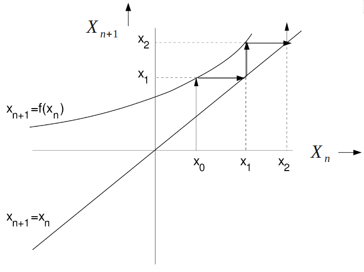
The cobweb plot will always have two lines on it, the \(X_{n+1} = X_n\) line, which is similar to a \(y=x\) line. The second line it will have is \(X_{n+1} = f(X_n)\). This line is the more curvy one, as it reflects the linear mapping that we do.
From here, we then draw a line from the bottom of the graph at some known \(X_0\) state to the second line we drew (the curvier one). From here, we obtain our \(X_1\). We can then draw a horizontal line across from that to the \(y=x\) line on the graph, then go up again to get \(X_2\).
The point of this is to create an analytical tool that helps us to understand the nonlinear dynamics of one-dimensional systems.
Non-Linear Difference Equations
Methods discussed so far yield analytical solutions to the problems. When we are studying non-linear equations, we have to move to numerical solutions.
In these systems, we can have things called equilibrium points, which are points where successive iterations do not change the solution. At these points \(X_t = X_{t+1}\), the system is in equilibrium and \(X\) is stationary. We can use superscript \(X_t^{\text{stat}}=X_{t+1}^{\text{stat}}\).
In the case of the logistic map, as we saw for modelling the rabbit population, this would be where \(X^{\text{stat}} = rX^{\text{stat}}(1-X^{\text{stat}})\). This can be solved with \(X^{\text{stat}} = 0\) or \(X^{\text{stat}} = 1\). Equilibrium points can be analysed without using analytical methods.
Stability Analysis
When we are using numerical algorithms, we need to see the convergence on or near an equilibrium point. If the numerical algorithm is not quite right, we'd ideally like to converge on the correct solution over time, and we want to avoid having a compound error.
Why do we do this?
In stability analysis, we upset the system a bit, and try to figure out the effect that this has on the system. In real terms, we linearise the equation around the equilibrium point, so something like the Taylor series approximation, then use the theory of linear maps that have been discussed above to see how stable the system is.
Fixed Points
A fixed point is where \(x^{\text{stat}} = f(x^{\text{stat}})\). This is the same as an equilibrium point, but could also be defined on a continuous function, as opposed to an iterative function. In some notation, \(x^{\text{stat}}\) can be called \(x^*\) instead.
Suppose there is a solution near that fixed point, at \(x_n = x^* + \eta_n\). Here, \(\eta\) is the distance from that stable point. Therefore, we can go through to the next iteration, and this will be:
As \(\eta\) is already small, the \(O(\eta^2)\) error will be tiny. With this term gone, we can then model the fixed point as a linearised map, which will have some multiplier \(\lambda = f'(x^{\text{stat}})\).
Using the properties from earlier in this lecture, we can then in constant time calculate \(\eta_n\) as \(\eta_n = \lambda^n \eta_0\). Using the derivative at the stationary point, we can see how stable the system is:
Stability Examples
Sine
If we define \(x_{n+1} = \sin x_n, x^{\text{stat}} = 0\), then \(\lambda = f'(0) = \cos(0) = 1\). From the earlier cases, we can see that the stability of this is marginal.
Cosine
For \(\cos\), we define \(x_{n+1} = \cos x_n, x^{\text{stat}} = 0.739\dots\). From here, we can see that \(\lambda = - f'(0.739\dots) = -\sin(0.739\dots) = -0.0129\dots\). Therefore, as we are less than 1, we are linearly stable.
Logistic Maps
So far, we have only looked at the stability of linear systems. If we look at the logistic map, the behaviour of the system dramatically changes, as this is a non-linear system.
Recall \(x_{n+1} = rx_n(1-x_n)\). Here, \(x_n\) is the population in some generation, and \(r\) is the growth rate of the population.
As \(r\) increases, we go from a fixed point, to a 2 cycle of different fixed points, then a 4-cycle, then 8, 16, 32, etc.
Periods (and Period Doubling)
Sometimes, these equations might become stable with a period of recurring solutions. In the instance of the logistic map, as we change \(r\), we obtain a cycle of \(2^n\). This cycle of \(2^n\) appears at a specific value of \(r\), and if we measure \(r\) when we start to see these cycles, as can be modelled with a computer, we obtain \(r_1 = 3\) for the 2-cycle, \(r_2 = 3.449\) for the 4-cycle, \(r_3 = 3.54409\) for the 8-cycle, \(r_4 = 3.5644\) for the 16-cycle, and an infinite cycle at \(r_{inf} = 3.569946\).
From the above, we can see that as \(r\) increases, the system gets to a point where there is no fixed point cycle. The values of \(r\) where each cycle starts converges to a final value.
Chaos
Where we have a high \(r\) value, such that it goes above \(r_{inf}\), we encounter aperiodic irregular system dynamics. In this system, not all \(r>r_{inf}\) are chaotic.
Bifurcation/Orbit Diagram
One way to visualise the chaos in the system is to plot a graph with \(r\) on the x-axis, and \(x\) on the y-axis. We can then plot \(x\) at some iteration based on a given \(r\) and observe the \(r\) at which the system goes from being linearly stable to a point where there are two stability points, then a point where there are 3 stability points.
The bifurcation diagram can be expanded into different bits as we narrow down the windows, e.g., for the logistic map function, we might go from \(0 < r < 4\) to \(3.8 < r < 4\), which would in essence zoom into that point.
Bear in mind that we can then do more iterations for each \(r\) we pick and model the state of the system more clearly. In a bifurcation diagram, we can normally see \(2^0\) to \(2^2\) and anything before becomes hard to deduce.
An example of a bifurcation diagram can be seen below (Wikipedia, author Biajojo, CC0):
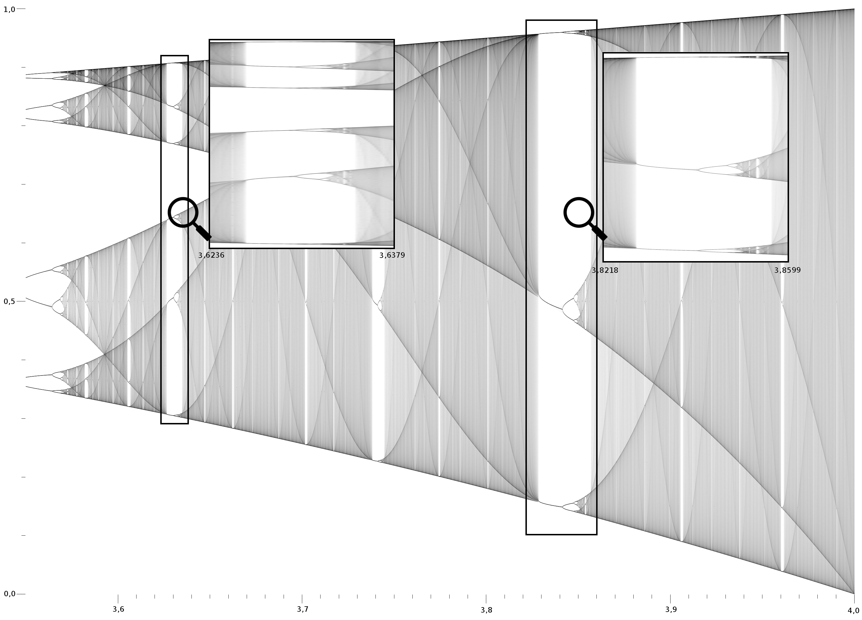
The bifurcation diagram for the logistic map looks poetic, with the emerging combinations of sinusoidal patterns. Bifurcation diagrams and stability are all parts of complexity theory.