Differential Equations
Note
This lecture has been done but is still a bit confusing. Future revision will be needed.
Differential equations have applications in things such as radioactive decay, population growth, chemical reactions, heat exchange, motion, etc.
They are commonly used in modelling and are a continuous analogue of discrete dynamical systems.
Differential equations are equations of an unknown function that involves some derivative of the unknown function. Newton's law of motion makes use of a differential equation. The law states:
The mass of an object times its acceleration is equal to the sum of the forces acting on it.
This is more commonly known as \(F = ma\). Acceleration is the first derivative of velocity: \(a = \frac{d}{dt} v\), and is the second derivative of position \(a = \frac{d^2}{dt^2}x\). If instead of defining \(F = ma\), we instead define it as \(F = m\frac{d^2}{dt^2}x\), then it becomes a differential equation.
Differential equations can be used to model the temporal evolution of any system.
Example: Malthusian Growth
Discrete Malthusian growth is modelled as a population \(P_n\) at some time \(n\) with a growth rate \(r\). This can then be modelled as a difference equation:
The change in population between the \(n+1\)st time and the \(n\)th time is proportional to \(r\) times the size of the population at time \(n\). This is because a fraction \(r\) of individuals has an offspring. Take e.g, \(P_0 = 1,r=0.1\), then \(P_1 = 1 + 0.1(1) = 1.1\), then \(P_2 = 1.1 + 0.1(1.1) = 1.11\), etc.
This also shows the interest on savings, which compounds over time. In this case, it gives \(P_n\) as the amount of savings at time \(n\), with \(r\) as the interest rate.
The equation shows that the savings next year will be equal to the savings this year plus the interest on last year's.
Another way we can visualise the growth of a population is to define \(P(t)\) as a function of the size of the population at time \(t\). We assume that \(r\) is the rate of change per unit time per individual in the population.
We introduce the notion of \(\Delta t\) as the small interval of time, with the change in population between \(t\) and \(t + \Delta t\) as satisfying:
This can be rearranged to give the following:
This is the discrete version of the model, as the time is specified in intervals. If we reimagine \(P(t)\) as \(f(x)\) and then \(\Delta t\) as h, the equation becomes:
As \(h \lim_{h\to 0}\), the equation takes the form:
This version of the equation is the continuous Malthusian growth model but expressed as a differential equation.
Solving
To solve a discrete system of the form \(P_{n+1} = P_n + rP_n\), we need to find a function \(P_n\) such that the equation meets some initial condition for \(P_0\) and permits us to answer the question given \(P_0\) at time zero, what is the size of the population \(P_n\) at time \(n\).
To solve an equation \(\frac{dx(t)}{dt} = f(x,t)\), which is normally expressed as \(\frac{d}{dx}f(x)\), we need to find a function \(x(t)\) that obeys the equation and meets some initial condition at zero time. This would imply that \(x(0) = X_0\).
This allows us to use a local rule to see how we progress from time \(t\) to time \(t+dt\), which then gives the global behaviour of the system.
Slope Fields
\(\frac{dy(x)}{dx}\) is the slope of \(y\) at position \(x\). Here, \(f(y,x)\) defines a slope or direction field. We define \(Y(x)\) as a function that is tangent to the slope field at every point.
Normally, we'd define a function in terms of \(f(x)\), then take the derivative as \(\frac{df}{dx}\) or \(f'(x)\).
The slope field is a function taking a point \((x,y)\) and returns the direction, or derivative of the function that we try and calculate.
Take, for example, the slope field for the function
This would create the following slope field (author Pbroks13, Wikipedia):
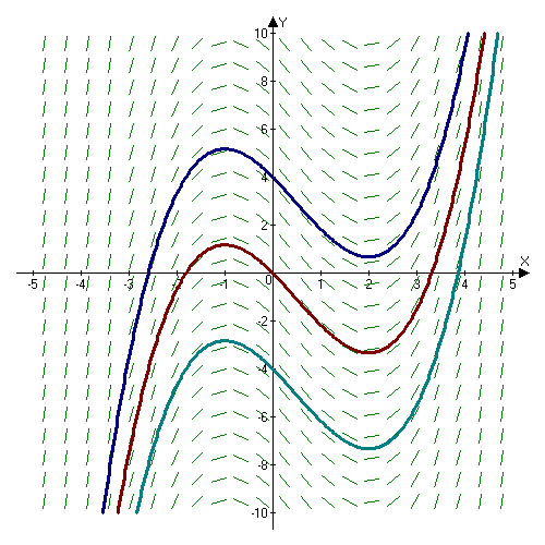
Within this image, the background lines give the gradient at some discrete points. These discrete points are solutions for the equation at given \((x,y)\), and as these are discretised, the space between each of these 'ticks' is chosen to be computationally feasible.
From this plot, we can take an initial \((x,y)\) for the system, then approximate a continuous function. For example, if we take \((x,y) = 0\), then we have the middle line giving the solution for the equation.
Example: Solving Malthusian Growth
As introduced earlier, the differential equation for continuous Malthusian growth is given with \(\frac{dP(t)}{dt} = rP(t), P(0) = P_0\).
We can then let \(c\) as an arbitrary constant with a solution of the form \(P(t) = ce^{rt}\).
If we then take the derivative with respect to \(t\), time, then we get:
Here, \(e\) is not a variable, but is the exponential function, and the derivative comes from the application of the chain rule. Here, we guessed that the solution for \(P(t)\) would be of the form \(ce^{rt}\).
From earlier, we can also show that \(\frac{d}{dt}P(t) = rP(t)\). Therefore, we know that \(P(t) = ce^{rt}\) solves the differential equation.
As we do not know the constant \(c\), we need to find the solution which obeys the condition that \(P(0) = P_0\) to find the actual solution. For this to happen, we show:
Therefore, the solution to the initial problem is \(P(t) = P_0 e^{rt}\), where \(r\) is the constant for the growth, \(P_0\) is the initial population, and \(t\) is the time delta.
Example: Find Solution and Determine Population Doubling Time
If we start with the model:
To find the time at which \(P(t) = 200\), we can substitute that \(P(t) = 200\), \(P_0 = 100\), and \(r=0.02\).
We can feed this into the forwards equation and get \(P(t) = 100e^{0.02 \times 34.657 = 199.99856 \approx 200}\).
Applications
Radioactive Decay
We let \(R(t)\) be the amount of some radioactive substance at time \(t\). Radioactive substances transition into another state at rate \(k \propto\) the amount of substance present.
The differential equation for this is \(\frac{dR(t)}{dt} = -kR(t)\), with an initial condition \(R(0) = R_0\). Analogous to Malthusian growth, the equation for \(R(t) = R_0 e^{-kt}\).
Harmonic Oscillator
A spring conforming to Hooke's law exerts a force proportional to the displacement of the spring. According to Newton's law of motion \(F = ma = -cx\), \(k^2 = c/m\), the simplest spring-mass problem is \(\frac{d^2}{dt^t}x + k^2x = 0\).
Swinging Pendulum
A pendulum is a mass which is attached at one point, swinging freely under the influsence of gravity. Given amplitude \(\theta\), Newton's law of motion gives \(\frac{d^2}{dt^t} \theta + \omega^2 \sin(\theta) = 0\), where \(\omega^2 = g/m\).
Logistic Growth
As discussed in the difference equations lecture, this is a better way to model populations. Most populations are limited by food, space, or waste and cannot continue to grow forever due to Malthusian growth.
Logistic growth has a Malthusian growth term, and a term which limits growth due to the crowding:
In this equation, \(P\) is the population size, \(r\) the growth rate and \(M\) the carrying capacity.
Lotka-Volterra Predator Prey Model
There is a population of prey \(x\) and predators \(y\) interacting in an ecosystem. They form a system of differential equations for \(x\) and \(y\):
There are no explicit solutions to this.
Classification
Differential equations are classified by their order, linearity, autonomy, whether they are ODEs (ordinary differential equations) or PDEs (partial differential equations).
Tip
Conversions are explained a bit badly here, my worked solutions to the problem sheets go through a few examples and explain a bit better. They can be found here (this one is week 5, sheet 4).
Order
The order is determined by the highest derivative in the equation. For Malthusian or logistic growth, these are 1st order, but harmonic oscillation is 2nd order.
The Lotka-Volterra model is a first order system of differential equations. Higher order equations can be transformed into systems of first order equations if we add new variables.
Reducing Higher Order to First Order
A harmonic oscillator is of the form \(\frac{d^2}{dt^2}x+k^2x = 0\). To reduce this, we introduce \(y = \frac{dx}{dt}\), giving \(\frac{dx}{dt} = y\) and \(\frac{dy}{dt} = \frac{d^2}{dt^2}x = -kx^2\).
This gives a system of two first order ODEs, which allows us to deal with systems of first order ODEs.
Linear vs. Nonlinear
A differential equation is linear is the unknown dependant variable and derivatives only appear in a linear manner. Here, Logistic growth, radioactive decay and harmonic oscillation are linear, but pendulums and the Lotka-Volterra model are nonlinear.
The differential equation is called autonomous because the rule doesn't care what time \(t\) it is. It only cares about the current value of the variable \(y\).
Autonomy
A differential equation is autonomous if there is no explicit dependence on time, e.g., \(\frac{d}{dt}x=x\) is autonomous, but \(\frac{d}{dt}x=xt\) is non-autonomous.
All equations presented above are autonomous, non-autonomous equations can be transformed into autonomous equations if we include time as an independent variable.
Conversions of Non-Autonomous to Autonomous
If we have \(\frac{d}{dt} x = xt\), then this is non-autonomous as it includes a reference to \(t\). If we set \(y = t\), and write \(\frac{d}{dt} y = 1\) in addition to substituting \(y\) into the equation to give \(\frac{d}{dt} x = xy\), then we have two autonomous equations.
Transformations
The above transformations from higher order to first order ODEs, and the conversion of non-autonomous to autonomous is reasonably simple to do. Much of the theory is only given for first order ODEs, and as higher order ODEs can be expressed as first order ODEs, it is redundant to give the theory in terms of both first order and higher order.
Furthermore, numerical solvers will often assume that we have systems of first order autonomous ODEs.
Partial Differential Equations (PDEs)
Differential equations can sometimes have unknown functions of multiple variables and their derivatives. The heat equation is given in terms of:
Where \(\alpha\) is the thermal diffusivity, \(\nabla\) comprises \(u_{xx} + u_{yy} + u_{zz}\), and \(u\) is the temperature field.
These types of equations are often solved numerically using methods such as finite difference.
Analytical Techniques for 1D
Before trying to solve an equation numerically, some analytical solutions do exist for 1D equations. When we solved the Malthusian growth equation, we guessed the solution. Instead of guessing, we can try to solve the equation in a more general way.
We move from the homogeneous case \(\frac{dx(t)}{dt}\) to the inhomogeneous case, \(a=Bx(t), x(0) = X_0\).
Example: Newton's Law of Cooling
After a murder, when a forensic scientist first arrives, they take the temperature of the victim, wait an hour, then take the temperature again. From these two datapoints, we can normally extrapolate the time of death.
This is because the body follows Newton's law of cooling, as the rate of change in temperature is proportional to the difference between the body's temperature \(T\) and the surrounding environmental temperature \(T_e\). This is expressed at:
Where \(k\) is some constant. If the victim is found at 0830 with a temperature of 30°C, then an hour later, they are at 22°C, with a temperature of the room at a constant 22 degrees, we can begin to solve the equation to yield the time of death.
We can use an ansatz to transform the equation, with \(z(t) = T - T_e\), and substitute that in to the initial equation.
This solution is now of the form \(z(t) = z_0e^{-kt}\). We can also see that \(T\) is just the environmental temperature plus \(z(t)\). If we now resubstitute into \(T(t)\), we get:
Because we have two unknowns \(t\) and \(k\). We solve this by substituting in \(30\) and \(28\) for our \(T(t)\) and \(T(t+1)\), taking \(T_0\) as the temperature initially:
If we then divide \((2)\) by \((1)\), we get:
To get \(t\), we can then insert either the value for \(e^{-k} = 6/8\) into \((1)\), or the value for \(k\), which I believe would be irrational. Inserting into \((1)\) we get:
So we get \(t = 2.19\) from our equation, and we subtract our time from the moment in time the first measurement was taken, which gives a time of death of 0830-0219 = 0611.
Falling Cats
If the environmental temperature differs, then we can't use the solution above, as that requires \(T_e\) to be constant. A better example for this is to look at the general case of a falling cat, as we can model the height, acceleration, etc.
Cats falling from a higher height will have more time to turn around and thus land on their feet. The main question we want to answer is whether the cat will land on its feet. Some important data we will need is that \(t_{turn} = 0.3s\). We want to deduce the minimum height a cat can fall from to land on its feet. We need the following:
This gives a second order differential equation. We need some sort of coordinate system to measure \(h\) as height, with \(h'' = -g\). For simplicity, we can assume that \(h(0) = H_0\), \(v(0) = h'(0) = 0\).
We then want to solve for \(H_0\) such that \(h(0.3) > 0\). To solve the equations, we can write them as a system of two first order equations:
To solve \(\frac{d}{dt} v = -g\), we see that the equation \(\frac{d}{dt}x = f(t)\) which gives some function on the RHS which doesn't depend on \(x\), only \(t\). We need a function \(x(t)\) which yields \(f(t)\) when differentiated.
This is called the fundamental theorem of differential integral calculus. This is showing that the integral is the reverse of the derivative. This integral will be:
In the case of the falling cat, this will be:
As we know \(v(0) = 0,t_0 = 0\), we get \(v(t) = -gt\). We now need to solve the second equation \(h' = v\), or \(\frac{d}{dt} h = -tg\). This equation is of the form \(\frac{d}{dt}x=f(t)\), so we can integrate again to get:
The critical point here is \(h(0.3) = 0\), so \(h_0 = g/2(0.3)^2 = 9.81/2(0.3)^2 = 0.44145m\).
Important Takeaway
If a 1D ODE is of the form \(\frac{d}{dt} x = f(t)\), and the RHS of the equation is independent of \(x\), then it can be solved by integration:
Modifying Malthusian Growth
the solutions discussed earlier are exponentials, of the form \(P(t) = P_0 \exp(r(t-t_0))\). The model works provided that there is some constant growth rate but fails to capture that growth rate will change with changing societal conditions:
Here, we have \(r(t) = a + bt\). For example, technology improves here and allows the population to grow faster.
Back to classification briefly, we can see that the model is still linear as both the unknown and derivatives appear in a linear manner, but is now non-autonomous, as there is a dependence on time in the function.
Modelling Census Data
Given the US Census data, is is possible to model the population from 1790 to 1990, provided we pick some \(a,b\). The right hand side is no longer purely a function of \(t\), as there is now a \(P(t)\) on the function.
If we have a differential equation of the form:
Then we can call it separable, as we can separate both \(x\) and \(t\) on the RHS. This can be written such that the LHS only depends on \(x\) and the RHS only depends on \(t\), by multiplying through by \(dt\), then dividing by \(N(x)\):
We can now integrate both the LHS and the RHS:
To model the Malthusian growth, which we can recall is of the form \(\frac{d}{dt}P(t) = rP(t)\), with \(r\) substituted for a continuous function \(r(t) = a + bt\), we get the following:
As with the earlier notes, we collect the like terms onto the same side of the equation:
Then, we take the integral of both sides:
Which, for the LHS is the same as \(\int \frac{1}{P}dP\). If we integrate \(1/P\), we get the natural logarithm of \(P\), and for the LHS, we increase the power of \(t\) and divide the term on the LHS by the new power:
Again, where \(c\) is some constant term. To then find the solution for \(P(t)\), we take the exponential of both sides:
We can then plot this on a graph with the given data to find a best fit of \(\log P\) to the census data, which will give us the parameters \(a = -7 \times 10^{-5},b=0.03476\).
Example: Solving Separable Equations
To differ from the last example, we can try and solve another equation \(\frac{dx}{dt} = 2tx^2\) in the same way:
General Linear Equations
The general formulation for a 1D differential equation is:
Which is linear if \(f\) is linear in \(y\). For this to hold true, \(f(x,y) = g(x) - p(x)y\), which is called the offset function.
Conventionally, these are notated slightly differently:
These types of equations can still be solved, but only for linear equations. The way we solve them is through the integrating factors method.
Integrating Factors Method
Useful Video
The lecture notes on this are confusing. See here for a good video that explains it well. This slide deck also came in handy.
We start with the differential equation of the form:
This looks like a total derivative, but it isn't quite because there is no function times the derivative and on the right there is no derivative either. To solve this issue, we can multiply both sides by a function \(\mu(x)\) to equal some RHS:
Only for some special values of \(\mu\) are we able to write the total derivative, and for this to hold, we need the following property:
If this works, then we can rewrite the equation as:
If this is the case, then the form of the equation has a RHS only dependant on \(x\) and a LHS only dependant on \(y\). If we can find a value of \(\mu\) that holds, then we could solve the differential equation by direct integration.
The difficulty is in finding a function for \(\mu(x)\) that holds. If we can find the \(\mu\) that holds, then we have a separable equation again, which can be solved as earlier.
The strategy to solve this is as follows: we first solve \((*)\) to find \(\mu(x)\) and then integrate \((**)\). We solve \((*)\):
From here, the second integral becomes:
This can be put all together such that the integrating factor is:
Note
We are not expected to remember this exponential, just how to get to this solution and derive it ourselves.
Example: Integrating \(\frac{dy}{dx}-2y/x = 0\)
We start with the following differential equation:
We identify \(p(x)\) as \(p(x) = \frac{-2}{x}\), then find our \(\mu\):
From here, we multiply both sides of \((***)\) by \(\mu(x)\):
As can be seen here, it is very difficult to analytically solve 1D linear differential equations. We are not expected to remember in huge detail exactly how it works, merely the idea of how it works.
The examples shown so far are already at the limit of how far we can go to solve them analytically.
Numerical Solutions
In the general case, analytical solutions are not available. Very often, we can develop numerical techniques to solve these, including numerical integration.
There are still some analytical methods for some classes of equation (e.g., systems of linear differential equations). In the bigger picture, we want to do some equilibrium analysis, to see where the system is stable, etc.
These will be covered in the next lecture.