Computer Vision Techniques
Computer vision is the process of deriving measurements that we can use for recognizing features. We also need to filter the images, both at a low level and a high level. Features can be perimeter-based, or area based. Perimeter-based focuses on the boundary or edge of the object, whilst area-based looks at the space enclosed by the boundaries.
Computer vision has lots of advanced techniques for feature extraction, which need to be compared and evaluated, with different techniques being suitable for different applications. The demonstrations and worksheets are modelled around the Feature Extraction & Image Processing for Computer Vision book.
Image Sampling
As part of extracting data from images which we can then use as features, we may wish to transfer our images from the spatial domain (e.g., brightness values, HSL, CMYK), into a frequency domain.
Fourier Transform
The Fourier transform is typically thought of in the application to audio, or signals processing, where the signal comprises many sine waves, at differing frequencies.
Here, \(\mathcal{F}\) refers to the Fourier transform, \(f\) is the function to extract the values at position \((x,y)\). \(N\) refers to the size of the input space in terms of pixels, and \(j\), unlike in a pure mathematics sense, is what we use to refer to for \(i = \sqrt{-1}\). This was the transform as understood by Fourier, but this decomposes, as we will see in a moment, into the modern 1D and 2D versions.
Continuous Application
The one-dimensional forward and reverse transformations are given below, with \(F\) for forwards and \(f\) for reverse, as the original function \(f\) is returned. Forwards: $$ F(u) = \frac{1}{\sqrt{2\pi}} \int_{-\infty}^{\infty} f(x) e^{-2\pi jux} \, dx $$ and reverse: $$ f(x) = \frac{1}{\sqrt{2\pi}} \int_{-\infty}^{\infty} F(u) e^{2\pi jux} \, du $$
In the above equation, we look at both \(x\) and \(u\). The \(x \in \mathbb{R}\) forms what are known as the variable in the spatial domain, and the \(u \in \mathbb{R}\) forms the variable in the frequency domain. These concepts also apply to Fourier transforms in two dimensions, as we will see in a minute.
Tip
The Fourier series was initially quite confusing, and both reading Chapter 2 in the textbook, and watching a couple of 3Blue1Brown videos on the subject (specifically this one) for a visual understanding proved to be quite useful.
2D Application
The Fourier transform can also be applied to a higher dimensioned space, in this instance 2D. The following formulas give the continuous definitions.
Discrete Application
The important takeaway from this is that the Fourier transform is simply a mapping from the time domain signals into the frequency domain. A typical Fourier transform works on continuous functions, which doesn't work for images, as these are stored as discrete sets of bytes. There is the Fourier series, and the discrete Fourier transform (often abbreviated DFT), which are used for discrete applications. Further to DFTs, we have the fast Fourier transform (denoted FFT), which is a faster way to compute the DFT.
The Fourier transform has both a forward transform, which maps from spatial coordinates into spatial frequencies, and a reverse transform, which is used to map back from the transform into the original spatial coordinates.
The 2D transform in the discrete space is similar to the continuous definition, but instead of integrals and a limit \(\to \infty\), we make use of sums and division over the entire space \(N\).
The following give the forward and inverse DFT for 2D space:
Amplitude and Phase
The Fourier transform is a complex transform, of the form \(z = a + ib\) both with a \(\Re(z) = a\) and \(\Im(z) = b\) part. When extracting possible features, we can store both the \(\Re\) and \(\Im\) parts, plotting them.
Thresholding
This is the oldest feature extraction technique from the 1970s. It is known as a single point operation, in that the pixels within the image are each evaluated alone. Histogram normalization is covered in the textbook as one of the main other points, and is the process of spreading the histogram of an image either across the spectrum based on intensities or the original histogram.
Thresholding, at the most basic level, is the process of assigning a 1 or a 0 to each pixel, based on if the intensity of that pixel meets a minimum threshold value. This can be set uniformly, which is where the threshold value is set at a specified level. Adaptive thresholding is the other main type of thresholding, with optimal thresholding, where the threshold value is selected as to separate the object from the background.
This implies the object has a different range of values to the background. The Otsu method automatically selects this, and this can produce quite a good result. Manual tuning may produce a better result in some applications, however.
Background Subtraction
The background of an image is not usually of use to us, as we want to focus on the object that is in the foreground. The most simple of these subtractions is to take a median of all the images, as it is unlikely that an object will occupy the same pixels for the entire duration of the capture.
More advanced methods, such as mixture of Gaussians, and more recently kernel methods (using convolutions) are other methods of subtracting the background.
Median Subtraction
This can be done in typically one of three ways. We can use temporal averaging, which is the straightforward averaging over time; spatiotemporal averaging, which accounts for both time and neighbouring points. Temporal median simply takes the median value.
Mixture of Gaussians
Warning
This section is unfinished at the moment, it might be revisited at a later date, but currently don't understand it well enough to finish it properly.
This is a method proposed by Stauffer and Grimson. The background is modelled with \(K\) independent Gaussian distributions, which are updated by an on-line method.
The lecture slides propose this in a one-dimensional view, where each pixel is represented by a single value, but in reality this is a vector. The set \(\{X_1, X_2, \dots, X_t\}\) models the history of different pixels, with each \(X_n\) modelling the current e.g., \(R\), \(G\) and \(B\) values of the pixels.
We can thus estimate the probability of each pixel intensity with \(K\) different distributions:
The weight \(\omega\) is adjusted over time according, where \(\alpha\) is selected as the learning rate, \(M_{k,t}\) is 1 where matched, 0 otherwise to the following formula: $$ \omega_{k,t} = (1-\alpha)\omega_{k,t-1} + \alpha(M_{k,t}) $$ In addition to this, \(\mu_t\), and \(\sigma^2_t\) are also updated.
Group Operators
Group operators work on multiple points at once, unlike the previous methods which are single point operations.
We use a matrix of values, known as a kernel, which works across the image in what is known as a convolution, to reduce the dimensions of the image, and perform useful things, such as edge extraction. The 3Blue1Brown video on this is really useful to providing an intuitive understanding of convolutions and how they apply to image processing, in addition to other fields such as probability.
A convolution is an operation \(*\), similar to multiplication \(\times, \cdot\), addition \(+\), division \(\div\) or subtraction \(-\). It can sometimes be confused for a multiplication.
The convolution of two continuous functions \(f\) and \(g\) would be \(f * g\). It can help to think in terms of discrete values initially, such as \(A=[a_1, a_2, \dots, a_n]\) and \(B=[b_1,b_2,\dots,b_n]\). To convolve these would produce a new array, where the elements of the array are defined as:
The output length of the "array" doesn't have the same size as pairwise addition, multiplication, etc. When working with images and kernels, it is common to chop off any terms of the resultant array, where not all elements of the kernel are included, e.g., not including the red aspects below:
The kernel may also be called a template. The original image is given in terms of \(p(x,y)\), with the new image as
The template or kernel is an \(m \times m\) grid, passing over an \(N \times N\) image. To compute the kernel naïvely, this would happen in \(O(N^2 \times m^2)\), but using the FFT, we can achieve this in \(O(\log N)\) time instead.
Convolutions can be computed using libraries such as SciPy or NumPy, with simple code:
import numpy as np
import scipy

np.convolve((1,2,3,4,5,6),(7,8,9))              # Naive, ~4.4s at 100kx100k
scipy.signal.fftconvolve((1,2,3,4,5,6),(7,8,9)) # Using FFT, ~400ms
Further considerations are what to do at the borders of the image (these are typically padded), the size of the kernel and image, and the speed of processing.
Statistical Filters
These are filters we can apply to the image. We have the mean, Gaussian average, and the median, which are all used to filter the images to make them possibly more suitable for processing.
Mean
These also act over an area \(m \times m\) pixels at a time. The mean is trivial to understand: $$ f(x,y) = \frac{1}{m^2} \sum_{i \in m} \sum_{j \in m} p(x,y) $$
Gaussian
The Gaussian average is slightly less trivial: $$ w(x,y) = e^{\frac{(x-x_0)^2 + (y-y_0)^2}{2\sigma^2}} $$ Here, \(x_0\) and \(y_0\) are the centre of the Gaussian function. \(\sigma\) is the standard deviation and controls the spread around the centre. \(e\) simply gives the function the standard bell shaped curve of the Gaussian distribution.
Whilst the function looks complicated, it is essentially a weighted average around the centre point, and can be applied similarly to the mean, working through a kernel of size \(m \times m\).
Median
This is the last of the simple techniques. The median is defined as: $$ f(x,y) = \text{middle}(\text{ranked}(p(x_1,y_1), \dots, p(x_m, y_m))) $$
The median reduces certain types of noise really well, and preserves edges in the data, unlike the Gaussian and mean which blur them. Unfortunately, it is relatively slow as we need to order the kernel, but is becoming more possible as hardware speeds increase.
Wavelets
Warning
This section also currently doesn't read perfectly, and some details could be improved or further clarity added.
Tip
There is a really, really good video on this for building up intuition here (34m). It is in a very similar style to 3Blue1Brown, and is produced by Artem Kirsanov. Watching this first before moving on is highly recommended!
Wavelets are recent additions to signal processing. They allow for decimation (the process of reducing the number of samples in a signal) in space and frequency simultaneously. This essentially means that we can describe an image in terms of frequency at a position, instead of the whole image.
Thanks to Heisenberg's uncertainty principle, we know that it is fundamentally impossible to have both the perfect time and frequency information, as \(\Delta f \Delta t \ge 1\).
At the time domain extreme, we can know the exact value of the function, but gain no frequency information; or at the other end, we can see the exact frequencies present, without seeing the exact temporal dynamics of these frequencies.
Wavelets sit in the middle between the time domain and the frequency domain. When doing time series analysis, it is inconvenient to look at the \(\sin\) function, as it is continuous and stretches to infinity. Therefore, we modify these functions, by restraining the function in time.
This is known as a wavelet transform, which is where we use wavelets to analyze the signal in the time domain. Wavelets are short-lived oscillations, which are localized in time. Wavelets are a family of functions, which each satisfy different needs. When discussing wavelets, we might not necessarily be discussing the same wavelet.
As a definition, a proper wavelet is a function \(\Psi(t)\), which satisfies two main constraints:
- the mean of the wavelet must be zero, i.e., \(\int_{-\infty}^{\infty} \Psi(t)dt = 0\), known as the admissibility condition; and
- the function has to have finite energy, such that squaring the curve, then integrating is some finite number, i.e., \(\int_{-\infty}^{\infty} |\Psi(t)|^2dt < \infty\).
To decompose the signal, we need to have a sinusoidal function of sorts, which we can convolve with the inbound signal, to determine how much of each signal is present.
The general formula for a wavelet can be modified, by turning both a time offset knob and a frequency multiplier knob. These are applied to the general functions as \(\Psi (\frac{t- b}{a})\), where \(t_0\) is the time offset of the wavelet, and \(a\) is the frequency offset. We label this \(\Psi_{a,b}\).
Morlet Wavelets
Note
Morlet wavelets aren't included in the slides, but help with the general understanding of the Gabor wavelet.
The general definition of the \(\Re\) part of a Morlet wavelet is a \(\cos\) function, which is dampened by a Gaussian bell curve:
$$ \Psi(t) = k_0 \cdot \cos(\omega t) \cdot e^{-t^2/2} $$ Here, \(k_0\) is the normalization constant, and as with earlier definitions, \(\omega\) is the frequency. The \(e^{-t^2/2}\) part is the Gaussian bell curve, which we use to scale the underlying \(\cos\) wave to make the wavelet satisfy the second property.
The actual definition of a Morlet wavelet is complex, and this is covered slightly later.
Wavelet Contribution to a Signal
At any point in time, the function \(y(t)\) can have a dot product with \(\Psi_{a,b}(t)\). This, in a one dimensional function is the process of multiplying the values together.
In higher dimensions, the dot product is generalised as:
Essentially, vectors that are similar have high positive values, vectors that are orthogonal have zero values, and vectors that are strongly dissimilar have high negative values.
To get the contribution of a wavelet \(\Psi_{a,b}(t)\) to the function \(y(t)\), we take the dot product, which then gives us a plot for the contribution over the time domain.
Following this, we can build up the notion of a function \(T\), which takes parameters \(a\) and \(b\), corresponding to the frequency amplification and time offset, respectively. We take the integral of the dot product with respect to time to get an idea of if the wavelet and function are broadly similar at time \(t\):
Now that we have an intuitive understanding of the wavelet function, we can exploit Euler's formula to get the wavelet in both the \(\Re\) and \(\Im\) parts, which gives us more information.
As a reminder, Euler's formula is: $$ e^{i\rho} = \cos \rho + i \sin \rho $$ where \(\rho\) is the angle.
Complex Definition of Morlet Wavelet
A Morlet wavelet is thus defined in terms of Euler's formula, with both the \(\Re\) and \(\Im\) parts:
This allows us to take both the real and imaginary convolutions of the signal across the domain, using many values of \(a\) and \(b\) to arrive at a set of outputs feeding into \(T(a,b)\). This then gives the intensity of the specified frequency at a given time. The \(\Re\) and \(\Im\) parts of these can be combined to create a vector with a distance from the origin, and this distance is what is used for the intensity.
We can plot these on a "scaleogram", typically using a colour for the third dimension.
Uncertainty Principle Violation?
This would seem to violate Heisenberg's uncertainty principle, as we can see both the time and frequency plots for the signal.
This is not the case, as is explained in the video linked above, the lower frequencies are spread out over a larger timescale, but allow us to see the frequency exactly. Bursty short frequencies are much less accurate in terms of the frequency but are plotted in terms of time very accurately.
Gabor Wavelets
These are very similar to Morlet wavelets, and the same two fundamental principles hold. The difference is very limited based on the function definitions, with there being a lack of the constant \(k_0\), and the start time \(t_0\) is similar to \(b\), and \(a\) does the same job.
Another slight difference is the way that the Gaussian bell curve falls off. The textbook and slides both give different definitions for the Gabor wavelet:
Play with a Gabor Wavelet
In Two Dimensions
If you really want to get confused, then you can apply the Gabor wavelet to 2D space. Similar to the regular wavelet, these are complex functions, with the formula:
The \(\Re\) part of this is the even part of the function, and \(\Im\) is the odd part.
Applications
Gabor wavelets can be applied to texture modelling and analysis, and they are used for things such as iris texture measurements, and face feature extractions for face recognition.
Intensity and Spatial Processing Techniques
Other aspects of processing can involve looking at the intensity of the image, and processes to normalize this to make further processing algorithms work better. Techniques to do this include histogram normalization, image scaling, and histogram stretching.
Histograms and Normalization
When analysing images, initially thinking in grayscale, we can create a histogram of the intensity on the \(x\)-axis and the number of pixels in the image with that intensity on the \(y\)-axis. Sometimes the image does not include any true blacks (an intensity of \(0\)), or any true whites (an intensity of, say, \(255\)).
In this instance, we can normalize the histogram, such that the entire histogram falls between \(0\) and \(1\), in terms of the grayscale on the \(x\)-axis, and in terms of the probability, such that \(\sum_{i=0}^x P(x_i) = 1\).
Image Scaling
Note
The lecture explains this in a very odd way with the use of a graph. We can do it without looking at the graph which transforms a histogram from \(x\) to \(y\), from \(0\) to \(255\). Simply think of the linear scaling as squashing the values into the \(0\le x \le255\) box, linear scaling with clipping as a similar squish, but without the entire original range, and the absolute value scaling as linear scaling, but anything below \(0\) starts to get brighter again.
Whilst it may seem that this would be to do with the size of the image in terms of dimensions, the slides initially discuss the ranges of the intensity of the grayscale aspects of the image. If they are outside of the typical range, we can do one of three things:
- linear scaling, where we adjust the values of the input to somewhere between the minimum and the maximum;
- linear scaling with clipping, where we apply linear scaling but clip certain outlier values from the scaling; and
- absolute value scaling, where we assign pixel values \(x\) to \(\frac{|x|}{\textrm{max}}\), where \(\textrm{max}\) is the maximum absolute pixel value. For pixels that are very negative in the original image, they would become very positive. The original blacks would remain black, but those below would start to become brighter.
In the slides, this is represented on a graph, where the input range is on the \(x\)-axis, and the output range is on the \(y\)-axis.
For a histogram with a minimum of \(-20\), and a maximum of \(300\), we can compute the equation of the line that passes through the line:
$$ \begin{align} x_A &= -20\ y_A &= 0 \ x_B &= 300 \ y_B &= 255 \ \frac{y - y_A}{x-x_A} &= \frac{y_B - y_A}{x_B - x_A}\ y &= \frac{255}{320}(x+20) \end{align} $$ Using this formula, we can then iterate across all the pixels in the original image to get an image where the pixels are in the correct range. We call these functions \(f : X \to Y\) transfer functions.
For a clipped image, this is similar, but the formula for the equation of \(y = mx+c\) differs in that \(y = 0\) for a certain range \(x<x_{min}\) and \(y=255\) for \(x > x_{max}\).
These also work for scaling when the original histogram is already within the bounds of the image. This is typically called histogram stretching.
Histogram Stretching
The histogram of an image may be too narrow, where the values of the raw data are broadly within a small range. We can scale to set the minimum of the stretched histogram to the lowest value registered on the histogram, and the maximum to the highest value on the histogram, which would increase the visibility.
This, however, still includes outlier values, which may not be that representative of the image. We can thus clip an arbitrary percentage of the values in the histogram, e.g., 5%, such that the range of the final histogram is much more even.
Edge Detection
Edge detection detects sharp changes in intensity within an image. Edges are broadly categorised into three main types:
- a step edge, where the intensity changes very distinctly between pixels (e.g., \(0 \to 255\)).
- a ramp edge, where the intensity changes over a certain number of pixels, and is gradual.
- a roof edge, where there are two edges very close to each other. This is sometimes called a ridge. This can sometimes also be a valley.
Finding an Edge
The best way to find an edge is to take a derivative. We can either detect the local maxima of the first derivative of an image, or detect the zero-crossings of the second derivative.
Taking the second derivative still has its issues though. The second derivative will also tend towards \(0\) when there is not much change in the value. We need to consider when it actually crosses the \(x\)-axis, not just when it is close to the \(x\)-axis.
The first derivative is useful for seeing the rise from low intensity to high intensity but it is at a local minima when on a falling edge (i.e., from high to low intensity).
The derivative as explained in the slides only works in one dimension initially, but can be generalised to 2D and higher dimensions as is covered later on.
Handling Noise
We have an issue if the image is noisy, as the gradient will constantly vary, unlike a continuous function, where the gradient will be smooth. This is because derivative functions are sensitive to noise.
Applying this to 2D
The examples seen thus far only handle functions with one dimension. The first derivative of images, which have a 2D domain corresponds to the gradient.
The formula for this in 2D is:
These are in the continuous domain, however, so we need to find a way to approximate them. We can make use of the good old convolution, as was discussed earlier, to create an approximation to these gradients.
The approximations are defined as follows:
Unfinished
This section on edge derivatives is incomplete, and may be wrong.
This is because \(\Delta\) is a vector of both the dimensions. When we take the derivative of \(\vec{\Delta}I\), \(\vec{\nabla} = [ \vec{i}, \vec{j} ]\), we have \(\frac{dI}{dx} = \lim_{x \to 0} \frac{I(x+dx,y) - I(x,y)}{dx} \approx \frac{I(x+1,y)-I(x,y)}{1}\). The 1 is because 1 is the smallest pixel size we can look at.
We can get this from looking at the image geometrically, where we have \([-1, 1]\), and this is applied to \(x,y\) with the gradient TODO
Different Kernels
Edge detection with simple convolutions may not work when the edge is not perfectly vertical or horizontal. We therefore have different masks, or kernels, which we can use to find edges instead.
Roberts
Roberts started with the filters/kernels we initially include. For an oriented edge, we apply the Roberts kernels, as these are an improvement where the edges are not horizontal, nor vertical:
Prewitt
Sobel
This is similar, but increases the smoothing property of the filter. It removes the noise first, then detects the edge.
In the slides, we have partial derivatives using Sobel masks. \(|I_x|\) means take the first derivative with respect to \(x\), \(|I_y|\) for with respect to \(y\), then \(|\nabla I|\) for derivative of both:
High Level Feature Extraction
Edges are what we call low-level or local features. There is another kind of feature, which is known as high level, or global features. This includes evidence gathering, active contours, statistical shapes, or skeletonisation and symmetry. To achieve this, we make use of template matching and the Hough transform. These are types of matching.
We can then extract features by evolution, using snakes, which are active contours. We then use statistical shape models, and things such as skeletonisation or symmetry. These high level features are at the image level, in comparison to the low level ones which are more at the pixel level.
Convolution vs. Correlation
We have previously discussed the concept of convolutions, or the \(*\) operator. This operator is used to convolve two continuous functions \(f\) and \(g\), such that \(f*g = h\). Convolution is defined as follows for continuous functions:
Correlation is similar to convolution byt has the \(\otimes\) operator, and is again performed on two continuous functions \(f\) and \(g\). We say the correlation of two continuous functions \(f\) and \(g\) is \(f \otimes g\). Correlation is similar to convolutions, with the only difference being that the \(f\) function is performed in terms of \(f(x'-x,y'-y)\) instead of as in convolutions. Therefore, the continuous definition of a correlation is:
In convolution we would typically flip the filter, but this is not necessary when using correlation.
Template Matching
Template matching is the simple process of correlating and convolving templates over an image. We start by positioning the template image which is a small sub image at \((0,0)\), then move it right and down to \((x-n,y-n)\). Where the brightness of the template image matches the brightness of the image, we add one to the score, then return the highest scoring area of the image.
This requires the template image to be the same size and orientation as it appears in the template, but this can be generalised to work on a template image that doesn't exactly match in shape or size.
On the slide for this, we are introduced to the formula \(\textbf{P} \otimes \textbf{T}\). This formula is known as the correlation of some image \(\textbf{P}\) with the template \(\textbf{T}\).
The correlation is found by first taking the Fourier transform of the image \(\textbf{P}\) and then multiplying it by the complex conjugate of \(F(\textbf{T})\). These are then converted back into the spatial domain after the cross product has been taken. This is done by using the inverse Fourier transform \(F^{-1}\).
The full formula in the continuous space would be given as follows, with the application in discrete space below:
With this calculation done, we get the correlation of \(\textbf{P}\) and \(\textbf{T}\), where a higher value means that we have better correlation. We can plot this in what is known as an accumulator space, or correlation map, which shows the points of high correlation with a higher intensity, and those with low correlation a lower intensity.
We can then filter this accumulator space with some sort of optimality criterion, to get the areas where there is high correlation, and thus it is likely the template falls at this location.
This is well visualized with a set of puzzle pieces and the location of a template piece within this overall puzzle. (Image reproduced from lecture slides, which originally adapted from Feature Extraction and Image Processing, Nixon & Aguado).
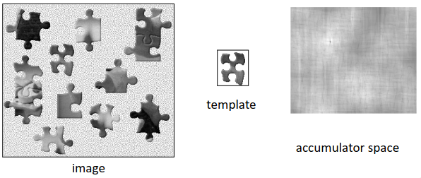
Whilst it is more intuitive to understand in the spatial domain, the Fourier transform method is substantially faster to run, and yields exactly the same result.
Hough Transform
This is another technique to detect a feature in an image. We may have a line that we want to detect within the image. We can use the Hough transform to detect this line in the image. This also works for other shapes.
In an image we may have a line. This line is in the \(x,y\) coordinate system. The line will have some equation \(y=mx+c\), where \(y,x\) are columns and rows. All we need to do is find \(m\) and \(c\) to find the line within the image.
If we choose a point on the line \(A=(1,1)\), then we have the equation \(y=mx+c\) must be valid at \(1=m+c\) (by substitution of 1 for \(x,y\)). We can then choose another point \(B\) on the line in the image, which will correspond to a line in the accumulator space \(c,m\).
For each point in the image, we will have some line in the accumulator space, as there are infinitely possible \(c,m\) that can determine the line.
For the Hough transform, we start with the original image, which we run edge detection on. This gives the edge map of the original image. We then create an accumulator space \(m,c\). This space is split into a finite number of cells. Each cell in the matrix has a value of zero initially.
To put a line with a given \(c,m\) into the accumulator space, we update the value of each cell the line passes through. In the edge map, we can then find the next pixel that is on the edge and get a new equation for \(m\) and \(c\) to get a new line.
This is repeated for all edges in the image, and at the end we will have lots of lines which have each been transformed into a map of cells. Within these cells, there will be boxes which have either no value or a low value. We can sort these values in the accumulator space with maximum first, then get the \(m,c\) coordinate of the first \(n\) maximum lines.
If we take the top \(n=2\) boxes, then we get the two most prominent lines in the image. By most prominent I mean the two longest lines in the image.
Problems
If we have an edge that is vertical, then the angle of the line is 90°, and so the slope of the edge would be 0, and \(m\) would become infinity. Therefore, the transform would fail if the edge is vertical.
To resolve this issue, we have to change the parameters we choose. We can tweak \(\rho\) and \(\theta\), where \(\rho\) (sometimes \(r\)) is the distance to the origin of the coordinate system from the line, and \(\theta\) is the angle. Instead of using \(c,m\) in the accumulator space, we end up using \(\rho,\theta\).
This is illustrated with the following image (Wikipedia, author Shcha, public domain):
If we use this for parameterisation of the line, then we avoid the issues with infinite gradients from vertical lines.
For Circles
Whilst the standard Hough transform can be used to detect the lines that are in an image, commonly from an edge map, it fails to find circles. Similar to the lines implementation, we start with an edge map, with a for loop until we get to a pixel that is on the edge.
As with the normal implementation, we also have to consider that the arc forming the circle may be incomplete, and that there are many disjoint arcs within the edge map forming the overall circle.
A pixel on the edge has values \(x\) and \(y\). In the equation of a circle, we have \(x,y,x_0,y_0\), which are the values of the current \((x,y)\) in the circle and the centre of the circle at \((x_0,y_0)\).
We can thus pass in the pixel value at \((x,y)\) to the equation, to generate the possible \((x_0,y_0)\) for the circle. Recall that the equation for a circle is: $$ (x-x_0)^2 + (y-y_0)^2 = R^2 $$
And substituting in e.g., \(x=3, y=7\) to the equation yields \((3-x_0)^2 + (7-y_0)^2 = R^2\). If we know \(R\), then we will only have two parameters which are unknown.
We then have an accumulator space, containing rows and columns which contain a set number of zero-initialized cells. In the accumulator space, any cell that this circle passes through is incremented by 1, with the rest staying at the value they were at before.
In the for loop, we can then move to the second pixel. We then plot the result of the second equation in the accumulator space too. Once finished, we can do the same thing as before, sorting the array and taking the maximums.
In the example above, we assume that we know the \(R\). This makes it easy to visualize the accumulator space for two dimensions. If we don't know \(R\), and most often we don't, then we plot a 3D accumulator space, with plots for \(R_{min} < R < R_{max}\).
In essence, this transform is the same as the initial transform, but uses parameters \(x_0,y_0\) instead of \(c,m\), or \(\rho,\theta\), but extends this 2D matrix into a 3D matrix, with differing values of \(R\) too.
Circle Voting and Accumulator Space
If we have \(0 < R < 10, R \in \mathbb{Z}\), then we have a 3D space. Where circles cross, we take a maximum to get the radius of the circle in 3D space.
Where the circles do not all cross at a point, we know that the \(R\) is likely wrong. Therefore, we can once again take the maximum, as this will be where the most circles cross.
Reducing Dimensionality of Accumulator Space
With the Hough transform, we were in 2D. With the circle transform, this increased to 3D. 3 dimensions takes longer to compute, and there is a method to reduce the complexity of looking at a 3D space.
To do this, we start with the equation of the circle, then take a derivative with respect to \(x\) on both sides of the equation:
For every pixel found in the edge map, we then need to find \(x,y,x_1,y_1,m\) which can then be sent into the differential. We then only have the two parameters in the accumulator space: \(y_0\) and \(R\).
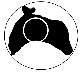
Active Contours
The Hough transform and its derivatives are useful for lines and circles. Active contours are used where we don't know the shape. Given some unknown arbitrary shape, we need to extract by evolution.
A contour consists of a set of points, with forces affecting the points. These forces pull the points about, until a point at which the forces are in equilibrium. We can think of the points as being connected with elastic bands, and a balloon in the middle.
Below, we can see how this evolves over time for an Iris detection.
Not Examined
On the slides for the module, definitions are given for a functional energy, internal energy, and an image energy. These are not expected to be known for the exam.
The algorithms are an optimisation problem that needs to be solved, where we try and minimise the energy.
Geometric
Active contours can either have points, or be a line, such as a circle, which over time will refine to a curve that segments something, e.g., a hand. This approach was introduced by Cremers, IJCV 2002. This generation of active contour is more advanced than the original active contours shown earlier, and yields better results. The paper also details a reference implementation.
Techniques for Object Description
Assuming we now have a segmented object, and we have the pixels inside that contour, we want to know what the object is. There are many different ways in which we can do this.
One way to do this is to set all pixels inside the contour to 1, with the rest of the pixels as 0. This is known as a segmentation map. To find something such as a hand, we have to find a way to represent the hand as a set of numbers, and then the computer can compare it to the numbers of another hand which is stored on the computer.
To find the numbers that represent the hand, we make use of either a region-based, or boundary-based technique. Region based looks at a black and white image, and we have to describe the black region with a set of numbers. Boundary based is where we only have the boundary and want to establish what the object is from just the boundary.
General Approach
We start with an image, extract features from the object (e.g., edge map), then extract some numbers, e.g., a histogram or something to get some numbers to represent the object. With these numbers, we can then train a classifier to either classify, match, label, correspond, recognize, or reason about the features.
Object description, and feature extraction in general are very important in many industries, including biometrics, surveillance, medicine, and industrial processes. The classifier will always try to find the best match in an image.
Normally, we have a dataset of objects, e.g., plane models, which is known as a database of descriptors. We train the classifier on this database. Then, when we have a new image, we calculate and compare the numbers to find the best match.
Applications: Target Detection
We train a classifier on a wing of an aircraft, also storing the best location to hit. If we then have an image of an aircraft, we can extract the features and perform matching, to locate the wings of the aircraft. As our trained model also includes the location of the target, we can see where would be best to hit.
Desirable Properties
An object description needs to have 4 properties in order to be a good descriptor. These are:
- Complete: different objects must have different descriptions
- Congruent: similar objects must have similar descriptors
- Compact: efficient, i.e., quantity of information
- Invariant: recognize independent of changes in e.g., illumination, and geometry (e.g., scale, translation, rotation)
Invariance is important as all we want to do is understand that an object is a specific object, and we don't generally care about the location of the object in an image, just what the object is. The four properties listed above will usually be put into a descriptor vector, which stores different objects.
Invariance
The most important aspect of invariance is to recognize independent of the orientation. This is fine in most cases, provided that there is no other object that exists that is a rotation of an object. E.g., in some fonts, \(M\) might be confused with \(W\), when rotated. Furthermore, \(M,W\) can also be confused with \(\Sigma\) in yet another orientation.
General Geometric Properties
Geometric properties are those related to purely the shape of the object, independent of its chromatic attributes. Examples of these properties include area, perimeter, compactness, dispersion, and moments (statistical). Once we have calculated these we can use them with a classifier.
Area
Given some binary image (e.g., 0s for background, 1s for foreground, or vice versa), the area can be given as such:
The area of a shape is invariant in translation and rotation, but not scale (a larger copy will have a higher area). This invariance will also not quite hold 100% as there are always small errors introduced when we discretise an image. For a set of shapes with the same resolution, we can assume that \(\Delta A\) is 1.
Perimeter
The perimeter of an object is the summation of the distances between consecutive pixels on the boundary of the object:
Here, each pixel in the perimeter is in \(P\), such that \(P_i = (x_i, y_i)\). The perimeter is also not scale invariant, but is translation and rotationally invariant.
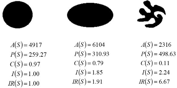
Compactness
This measures the efficiency with which a boundary encloses an area. This is defined as:
which can be written as:
Where the lower half of the fraction gives the area of a circle with perimeter \(P(s)\). This is invariant in the three properties (scale, translation, and rotation). Due to this invariance, it is a very good feature to use for classification.
The compactness of a circle is always one, and the compactness of any other shape is always less than one, but will always be bigger than 0. Additionally, for a shape with a perimeter \(p\), there will always be a circle with the same perimeter \(p\), but the circle will always have a larger area, provided that the shape is not also a circle.
If the shape of the object is almost a circle (i.e., an ellipse or similar), then the compactness (\(C\)) of the shape will be close to 1.
Dispersion
Dispersion measures the occupancy as the ratio between the area of the circle enclosing the region and the area of the region. Dispersion is defined as:
This is invariant in all three properties.
Alternatively, we can define dispersion as the ratio between the circle enclosing and the area of the circle contained inside the region. The first definition can be captured as follows (ignoring the blue lines):
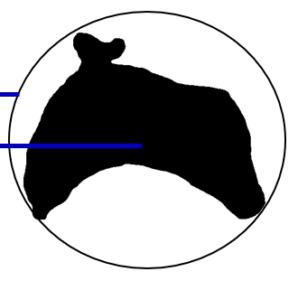
and the second, with the inner circle given in white:
Images from lecture notes. The second definition can also be captured mathematically, and holds the same three properties:
Moments
These can also be used as descriptors or features to describe a shape. They are defined with the following equation:
These are known as geometrical moments, but there are a range of different types, dependent on which polynomials we use (the \(p,q\)). For a zero-order moment, giving the total mass, this is defined as:
Zero Order
For binary regions, the mass corresponds to the area of the shape (in the above equation, we see that \(m_{0,0} = A(s)\).
Moments were initially introduced in physics and mechanics, with the moments assigned to objects with masses. In our implementation, we are looking at images, but we borrow the physics word for this, meaning that instead of the area, we say it is the total mass of the shape.
First Order/Centre of Mass
This is \(m_{1,0}\) and \(m_{0,1}\):
These can be combined with the zero order moment to get the location of the centre of mass, which we define as being at \((\bar{x},\bar{y})\):
Moments of a shape are only invariant in \(m_{0,0}\), in the same way that area is. A general moment of the form \(m_{p,q}\) is not scale, translation or rotationally invariant.
Translationally invariant moments are called centralised moments, translation and scale invariant moments are called normalised central moments, and translation, scale, and rotationally invariant moments are simply called invariant moments.
We make them invariant in translation, then scale, then rotation so they can be used as features for classification.
Centralised Moments
These are defined as follows, and translate the image to the origin:
First Order
First order centralised moments \(\mu_{1,0}\) can be derived from the definition of \(\bar{x}\), such that we eventually get \(\mu_{1,0} = 0\). This is derived in more detail in the lecture slides.
Second Order
This derivation is more complicated but we go from \(\mu_{2,0} = \sum_x \sum_y (x-\bar{x})^2 I(x,y) \Delta A\) to \(\mu_{2,0} = m_{2,0} - \frac{m^2_{1,0}}{m_{0,0}}\). Again, this is given in full detail in the lecture slides.
Second order moments for the following shapes have been calculated and are listed below (again, from the lecture slides):
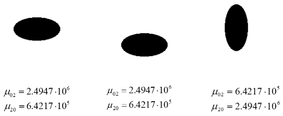
This shows that for the same shape, the second order centralised moments are only invariant to translation, but not to scaling or rotation.
Normalized Centralised Moments
Sometimes the image may be scaled, and the object in one image is bigger or smaller than in another image. We want the system to continue to be able to recognize the object.
The normalized central moment of order \(p + q\) can be found by dividing the central moment of the same order by some normalization factor. We have \(x' = kx\) and \(y' = ky\).
The noramlized centralised moment is given in terms of
This is noramlized because the centralized moments are divided by a coefficient. The process of division is known as noramlization.
The reason for the bounds on the \(p+q\) is to ensure that we have a centralized moment that is not zero.
Second Order Normalized Central Moments
Similar to a second order central moment, the second order normalized centralized moments are of the form:
These moments are now invariant to the position and size of the object. The third and final stage is to make the moment invariant to rotation. The maths for this is much more complicated, but has been published in papers as early as the 1960s.
Invariant Moments
There is a paper which gives moments \(M1\dots M7\), which will stay the same regardless of whether the image is rotated, in addition to whether the image is scaled or translated.
One such moment is known as the Hu moment, and is given as \(M1\):
Proving Rotational Invariance
It is possible to prove that the moment is invariant with resepct to rotation, by considering the shape in the origin, such that \(\bar{x}, \bar{y} = 0\). This is used for simplicity of the proof.
If both \(\bar{x},\bar{y} = 0\), then calculation of \(\mu_{20}\) and \(\mu_{02}\) becomes easier as we no longer have to include those terms in the equations, as they will be \(\pm 0\).
Therefore, the equations become:
We can then substitute into the original equation for \(M1\), to give:
So for \(M1\) to be invariant, we have to prove that the numerator of the fraction above is invariant with respect to rotation.
One way we can do this is to instead of rotating the shape, rotate the coordinate system instead. The coordinate system is rotated by an angle of \(\rho\) (because why not not use \(\theta\)). We can then assume that the shape remains unchanged, despite it changing in the new coordinate system.
If we take a coordinate of a shape to be at \([x,y]^T\) in the original coordinate system, then apply a rotation \(R\), so we get \([x', y']^T = R[x, y]^T\), we translate the coordinates into the new system.
Recall that for a rotation, we can define \(x'\) as \(x \cos \rho - y \sin \rho\), and \(y' = x \sin \rho + y \cos \rho\). This is normally written as a left multiplication of a \(2 \times 2\) matrix, but has been linearised in the lecture slides.
From here, we can add this \(R\) in its constituent aspects alongside the \(x^2\) and \(y^2\) terms:
Expanding out these terms yields \(x^2\cos^2 \rho + x^2\sin^2 \rho\) for the \(x^2\) term, which once pulling out \(x^2\) yields \(\cos^2 \rho + \sin^2 \rho\). This is the identity for sine and cosine squares and will always equal one.
Similarly, the \(y^2\) terms also cancel out with the identity, and the non-squared terms as a consequence end up cancelling out. Therefore, the equation can be simplified such that we end up with
thus proving that these are rotationally invariant. (QED, or whatever, I guess).
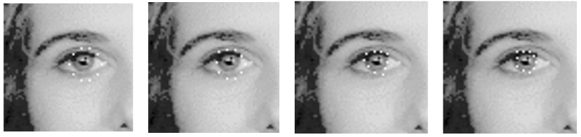
Invariant moments for three images, the first two of which are the same, and the third of which is different are given below, along with the images (reproduced from lecture slides):
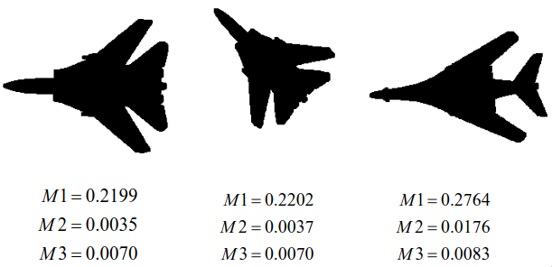
Here, we can see that \(M1\dots M3\) are broadly the same, save a couple of truncation errors for the first two, with the moment for the third image being quite different, besides being a similar shape to the eye.
Again, all three of these moments can be fed into a classifier as data to aid the classifier in its job.
Overall Advantages and Disadvantages
Moments work well on greyscale and binary objects. They can make use of the pixel brightness (the \(I\) function), and have access to lots of detail within the image.
Issues with them include that they assume only one object, they are computationally quite expensive, and higher order moments create large numbers, which can be sensitive to noise. Of course, a good classifier should not put as much weighting on a moment that is susceptible to noise, but use it as a part of a heuristic.
Invariance Comparison
| Property | Scale | Translation | Rotation | Bounds |
|---|---|---|---|---|
| Area \(A\) | ✗ | ✓ | ✓ | \(>0\) |
| Perimeter \(P\) | ✗ | ✓ | ✓ | \(>0\) |
| Compactness \(C\) | ✓ | ✓ | ✓ | \(0 < C(s) \le 1\) |
| Dispersion \(I,IR\) | ✓ | ✓ | ✓ | |
| Zero Order Moments \(m_{0,0}\) | ✗ | ✓ | ✓ | |
| General Moments \(m_{p,q}\) | ✗ | ✗ | ✗ | |
| Centralised Moments \(\mu_{p,q}\) | ✗ | ✓ | ✗ | |
| Normalized Central Moments | ✓ | ✓ | ✗ | |
| Invariant Moments | ✓ | ✓ | ✓ |
Shape Description
Another type of shape description we can do is based on the boundary of the shape. Methods for this are broken down into discrete: chain codes, run length codes, and extreme points; curves: polynomials, splines, wavelets, Fourier; and properties: length, curvature, bending energy, and convexity.
Fourier Descriptors
The general framework is to take a template of an object, and a picture of a real object. Initially we compute a boundary, then use a Fourier expansion to calculate the Fourier coefficients, then calculate Fourier descriptors based on these calculations.
For the same object, the Fourier descriptors should be the same, even though the Fourier expansion/coefficients might not be the same. As with moments, the Fourier descriptors are built up from the Fourier expansion by making them invariant to the main properties.
Fourier descriptors have many different types, and at each stage of curve extraction, Fourier expansion, and Fourier descriptors, there are many ways to do the same job.
Curve Extraction
Curves can be represented with polar coordinates, a radial distance function, a speed function, a tangent vector, a tangent contour, or a curvature vector function. These are all differing ways that we can represent the curve.
The main options that we choose are trigonometric, or elliptic. The first of these approaches is the polar Fourier descriptors, which make use of a cumulative angular function and the Fourier series in trigonometric form.
The latter is the elliptic Fourier descriptor which creates a complex curve and uses the complex and trigonometric forms of the Fourier series.
Elliptic Approach
The basic approach here is to obtain some complex function from the 2D curve, perform a Fourier expansion and then define descriptors from Fourier coefficients.
Complex curves have the form:
Again, for some reason we use \(j\) instead of \(i\) for the imaginary number \(j = i = \sqrt{-1}\). Instead of imagining the coordinate system as \((x,y)\), we imagine it as \((\Re, \Im)\), with the contour \(c\) as a component of its real valued part at time \(t\) and its imaginary valued part at the same time. We call \(t\) the parameter.
Once we have this complex valued function, we can write the Fourier transform as:
This form is known as the Granlund form, with the coefficients known as the Fourier coefficients. This is an approximation of the Fourier transform.
There is also a trigonometric version, known as the Kuhl form:
For a trigonometric expansion of \(c(t)\), we perform the expansion on both \(x(t)\) and \(y(t)\), so we have four sets of coefficients \(a_{xk}, a_{yk}, b_{xk}, b_{yk}\), which are the Fourier coefficients for zero-frequency.
The way to find these coefficients is to make use of the following equations (known as the Fourier equations):
For those parameters with \(x\), we have \(x\) in the integration, and for the parameters with \(y\), we have \(y\) in the integration.
Substituting in these expansions to the \(c(t)\), we get:
or, in matrix form:
As with when the Fourier transform was introduced, we also had to have a discrete version, for when the functions were not continuous. In this instance, our parameters change from the trigonometric form, as above, to the discrete form:
Extracting Fourier Descriptors
So far, we have established how to extract Fourier coefficients. We now adapt the coefficients and try to make them invariant, as with our moments earlier.
If we have a contour that can be represented as a Fourier series, we can give it the invariant descriptors as listed above:
Translation Invariance
If this is then translated across the screen, then we end up with
or,
The only difference that we can see is in the zero frequencies. Frequencies dependent on \(k\) are not affected by this translation. If we ignore the zero frequencies then the Fourier descriptors become translation invariant.
Because of this, we can say that:
Scale Invariance
To scale the curve would be to apply a scaling factor \(s\) over the summation of the \(k\) terms:
We can introduce the notion of \(a'_{mn} = sa_{mn}\) where \(mn \in \{x,y,k\}\). If we scale the contour, for the descriptor to be scale invariant, we need to have:
Rotational Invariance
Given an original contour
The rotation of this would be:
To make it rotationally invariant, you guessed it, we need to pick \(x'_{mn}\) which are equal so some version of \(x_{mn}\). For these, we need to ensure the following properties align:
Missing bit for derivation of orthonormal property and invariant descriptors, need to somehow add examples
We give the descriptors to the classifier for training and recognition, as parameters. These are a differnt approach to moments, as they are boundary based as opposed to region based. Dependent on the application, we may have better results with moments, or Elliptic Fourier descriptions.
Discretising the Fourier Descriptors (Multiscale)
Initially, we use \(k\) in the range from \([-\infty,\infty]\), but this is not possible, as computers work in discrete time, and do not have infinite memory (as opposed to what Chrome believes).
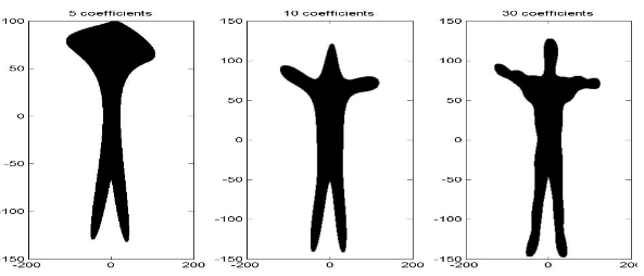
Computers should have a limited number of frequencies and thus a limited number of descriptors. The number of descriptors to choose increases the number of details captured, and the histogram plot for these will reveal more nuanced details the further away from the \(y\)-axis we are.
If, instead of choosing \(\sum_{k=1}^\infty\), we have \(\sum_{k=1}^n\), then we can capture different amounts of detail from the contours. Below, there are images for a captured contour for \(n=5,10,30\) coefficients:
Summary
Object description is a fundamental problem in image processing and computer vision. Broadly, it is split into two categories: regions (e.g., moments); and borders (e.g., Elliptic Fourier Descriptors).
The most difficult problem is in the evaluation of these techniques, and typically, we look at the performance within the application (e.g., correct classification, time costs for inference).
Classification
There are lots of applications for classification. Classification is the process of separation of objects into categories of similar types. Classification algorithms will put similar objects into similar groups.
Classification has applications in face recognition, remote sensing, and object recognition, to name a few. These groupings are managed by a system known as a classifier.
A classifier, ideally, would take a group of images of things and group them such that one group it classifies is one thing.
Before we can classify, we need to try and extract features from the image. For image recognition tasks, this is usually the greyscale of the image.
Similarity
To quantify when two images are similar, we need to look at their pixel values. We can say that two images \(I_1,I_2\) are similar when either their absolute difference \(|I_1 - I_2|\) or \((I_1 - I_2)^2\) is small. A simple feature would be the intensity of the pixel in a \(1\times 1\) grid.
If we expand this image to have a size of 2 pixels by 1 pixel, then we can have two features, \(f_1,f_2\). The feature \(f_1(I) = I(1,1)\) and \(f_2(I) = I(1,2)\). These features can then be made into a feature space, which is a graph of each feature on each axis, with the image each representing a single point. For a 1x1 image, the feature space is 1D, for 2 pixels, it's 2D and for 100 features it would become 100D.
To extract the similarity between images within a feature space, we take the distance between the two. For an \(N\times N\) image, the feature space would be \(N^2\) in dimension. Therefore, a notion of the distance in a high-dimensional space is required (similar to Manhattan distance and Euclidean distance in 2D, that we are familiar with).
The Manhattan distance in an \(N^2\) dimensional space, this would be:
And the Euclidean distance:
These are known as metrics. Metrics must satisfy three conditions for a measure to be a metric. These are:
- \(D(a,b) > 0\)
- \(D(a,b) = D(b,a)\)
- \(D(a,c) \le D(a,b) + D(b,c)\)
If the distance metric meets these conditions, then it can be used by the classifier or the classification algorithm.
Features
In practice, we cannot use pixels as features as they take up lots of memory and CPU for any reasonable sized image. E.g., for an image with 100x100 pixels, we would have a 10000 dimension feature space. This is 'a recipe for disaster'. As the dimension of the feature space increases, the accuracy will go down.
Therefore, instead of pixels, we make use of other features. These might include moments, area, compactness, Fourier descriptors, etc. These represent or describe the object inside the image, whilst at the same time reduces the dimensionality of the feature space and thus increase the accuracy of the recognition system.
Training a Classifier: Multiple Images
If we have now taken images and processed their features, to output them to a feature space, we'd hope to see some sort of clustering between images that are similar. Clustering is easily visualized in 2D space (and possibly 3D at a stretch). Once these groupings have been created, we can then either classify them by hand, which is known as supervised learning (with something such as \(k\) nearest neighbours), or an unsupervised technique called \(k\) means clustering.
Supervised Learning
The first approach is where we have a collection of known images, known as the training data. We train the classifier with this training data, telling it that images with these specific features belong to this class.
When we encounter an unknown image (test image), we want to try and establish which class the image belongs to. The training data is what teaches the classifier.
K Nearest Neighbour (KNN)
This is a supervised classifier, requiring the training dataset. The way it works is that it takes \(k\) nearest neighbours, and the algorithm computes the distance from all other points (neighbours). We then sort the distances from the shortest to longest, then pick the nearest \(k\) elements. From these elements, we then vote on these \(k\) examples as to the class the image belongs to.
If we have an even \(k\) and there is a tie in the number of votes, then we go by the shortest distance.
Unsupervised Learning
On the contrary to supervised learning, unsupervised doesn't know what the class of the data is in the training dataset. Given a collection of examples, we want to group them into classes based on their features.
The good thing is that we don't need to train the algorithm, per se. Classification is done with the K means clustering algorithm.
K Means Clustering
We try to represent the data by \(k\) centres. We aim to minimise \(J = \sum_{j=1}^K \sum_{i \in S_j} D(I_i, \mu_j)\). One thing we have to do is tell the algorithm the number of groups it should expect.
The algorithm chooses some \(k\), then randomly assigns examples to one of the \(k\) sets, compute the mean value for each set \(\mu_j\). We then reassign each point to the nearest mean, then repeat from the mean value computation until the mean values remain unchanged.
Cumulative Match Curves
No Recording
In the recording that covers this slide, he says that we already discussed CMCs, but I cannot find a recording of this. From here to the end of FRR and FAR, the lecture recording did not capture the whiteboard very well, so this bit is missing some details.
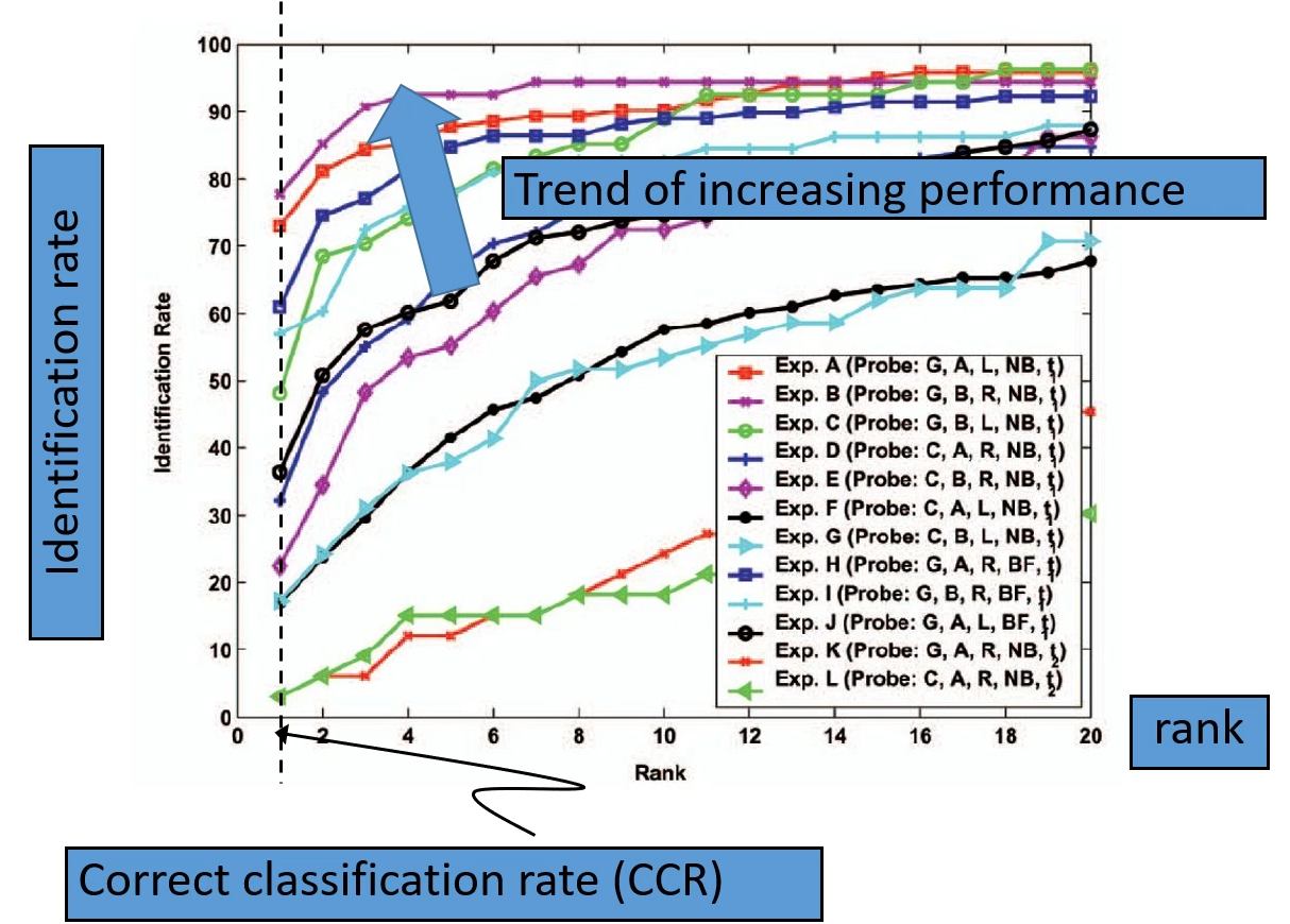
Horizontal axis is the rank, and the vertical axis is the identification rate or the correct recognition rate. If the curve approaches the top of the coordinate system, then it shows that the system is performing better than the other systems. The correct recognition rate (CRR) is the ratio of correctly recognized subjects divided by the total number of the subjects:
The rank is an ordered list of subject recognition. The lowest rank corresponds to the shortest distance or highest probability, and the highest rank corresponds to the highest distance or lowest probability. We make use of the rank in the CRR, by using the correct subjects at rank 1.
Intra/Inter Class Variation Plots
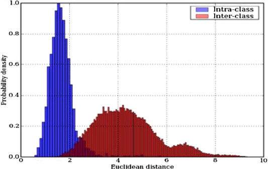
This is a histogram that plots two series. The first series is the intra-class variation, and the second is the inter-class variation. The plot has the Euclidean distance on the \(x\)-axis and the probability density on the \(y\)-axis. As we have the probability density, it is normalized. The distances are computed between all points.
In the image, the taller series shows that within the same class, there is little variation in the distance. The second, more spread out series on the diagram gives the distance between different classes, and the further to the right that is, the better separation there is between different subjects.
Where there is overlap between the two series, then we have confusion, and the performance of the classifier is reduced. This is called the confusion region. Therefore, this plot is good to use to see what the performance of our classifier is likely to be.
When classifying, everything that is in the blue-red area would be a false positive because it would have been incorrectly accepted by the blue.
The true positive is put in the \(y\)-axis and the false positive is put in the \(x\)-axis, then we define a threshold, which we change and gradually increase. We can choose where to put the threshold, such that anything on the left of it would be true positive, and we can tune to a false positive rate. If we place the threshold at a point where inter-class variation is zero in terms of the density, then our false positive rate will be almost nothing. On the other hand, there is still quite a lot of the histogram for the intra-class variation which would then fall on the wrong side of the threshold and would thus be classed as false-negative.
Increasing the threshold increases the true positive rate, but also increases the false positive rate. The plot for this therefore becomes:
In summary, a high threshold ensures a low false positive, a medium threshold strikes a balance between true positive and false positives, and a low threshold increases both the true positive and false positive rates.
ROC Curves
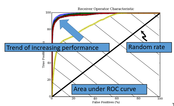
A ROC curve, or a receiver operator curve is used not only to show the performance of the classifier, but gives information on the feature extraction and the dataset itself.
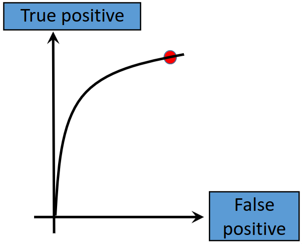
A ROC curve plots the false positives rate (\(x\)-axis) against the true positives rate (\(y\)-axis). The ROC curve for random data will span a line from \((0,0)\) to \((100,100)\). As performance increases, the curves will begin to approach the top left corner.
The problem with the methods so far is that there is a dependency of accuracy on the threshold. We can therefore say that the accuracy increases or decreases as we move the threshold. A better way to show the 'accuracy' or performance is to take the area under the ROC curve, as this does not vary with the threshold. ROC curves show the error of the system, instead of the accuracy.
FRR and FAR
FRR is the false reject rate, or false negative; and FAR is the false accept rate, or false positive. These are used to quantify error instead of accuracy.
Choosing a high threshold means that we have a high FRR, and a very low FAR. As the threshold decreases, the FRR decreases and the FAR increases, giving roughly equal error. Towards the other end of the threshold, where we have a low threshold, then we have a low false reject rate. Where the curve is in the middle, we call it the equal error rate.