Elliptic Curve Cryptography
Elliptic curves are specific forms of curves that are 150 years old. They were first proposed for use in cryptosystems in 1985 independently by Neal Koblitz, and Victor Miller.
In the 1990s, they were standardized by a number of organizations, and began to be used. As with other cryptosystems, the length of the keys required has increased dramatically, but ECC systems still require shorter keys than conventional, e.g., RSA. The main reason for standardization was that ECC required less resources and energy, and RSA was a much 'heavier' protocol.
Definition
Elliptic curves \(E\) are defined as a graph of the equation of the form:
Simple Elliptic Curve Demo
The type of curve we are interested in for cryptographic purposes contains two separate parts, a circle-like shape on the left, and then a line-like shape on the right.
In addition to the equation above, for cryptographic purposes, we need to add a point at infinity. Besides the demo above, we can see that the shape of the curve changes with different \(a,b\).
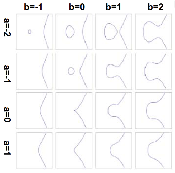
The curves above show the two main variations: those that have the separate shapes, and those that form one continuous line.
Restrictions
Given the polynomial \(x^3 + ax + b\), we have some curves which have a double root. This cannot be used to construct a cryptosystem. We can therefore add the restriction that \(4a^3 + 27b^2 \ne 0\). We use this restriction to ensure that the EC equation has three distinct roots.
Abelian Group Structure
ECC permits a natural Abelian group structure. Recall that a group is a set of numbers, and an operation. This set of numbers, for ECC, is a set of numbers that can create a curve. For example, let's do it over the real field \(F = \mathbb{R}\). This makes it easier later when we want to show the group structure over some modulus \(\mathbb{Z}_n\).
Closure over \(\mathbb{R}\)
Addition Where \(P \ne -Q\)
If we have \(P,Q\) as distinct points on a line that passes through the circle bit of the elliptic curve (restriction \(P \ne -Q\)), we can show addition over closure. This line will intersect the curve in precisely one more point on the 'arc' bit of the curve, which we call \(-R\). We then take a reflection of this point in the \(x\)-axis to get \(R\). Visually:
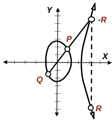
Following this, we therefore define addition in an elliptic curve group as $$ P + Q = R $$
We can establish \((x_R,y_R)\) with the following:
We can then define \(x_R\) and \(y_R\), making use of a \(\lambda\) term to help as:
Proof
To find \(R\), we need to solve the following equations:
Substituting \((2)\) into \((1)\) yields:
$$ (y_1 + \lambda(x-x_1))^2 = x^3 + ax + b $$ which can be reduced to a form of \(x^3 - m^2x^2 + \cdots = 0\). The sum of the three roots is then equal to \(-(-m_2) = m_2\), and we know \(x_1,x_2\) are roots as \(P,Q\) is on the curve, giving the third root as \(x_3 = m^2 - x_1 - x_2\).
We then substitute \(x = x_3\) in \((2)\), to yield:
Thus, we have \(R = (x_3, y_3)\) and can define addition \(P+Q\) as:
Addition Where \(P = -P\)
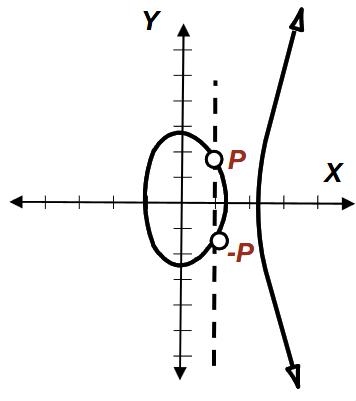
In the case we have \(P=-P\), the line is vertical through the circle bit, and thus will never intercept the curve at a third point. We cannot, therefore, add in the same way as before, as there will never be a third root on the curve.
To solve this small problem, we introduce the notion of \(O\), which is a point at \((\infty, \infty)\). We can then define definition of \(P + (-P)\) as \(O\).
This would give the following graph:
One interesting note here is that we can rearrange \(P + (-P) = O\) to get \(P + O = P\), which shows that \(O\) is some sort of additive identity over the elliptic curve group.
Doubling a Point Where \(y_P \ne 0\)
We have two special cases to double a point. Where \(y_P\) is not equal to zero, the tangent to the curve will not be vertical. Therefore, the tangent line will pass through the curve at \(-R\), which is the reflection of \(R\) with respect to the \(x\)-axis.
By definition of addition, \(P + P = 2P = R\).
Proof
In the case \(y_P \ne 0\), we have \(P = (x_1, y_1)\), \(2P = R = (x_R, y_R)\), where \(x_R = \lambda^2 - 2x_1\), \(y_R = -y_1 + \lambda(x_1 - x_R)\), given \(\lambda = \frac{3x_1^2 + a}{2y_1}\).
Doubling a Point Where \(y_P = 0\)
In the case \(y_P = 0\), then by definition, the tangent line on the EC at \(P\) is vertical and doesn't intersect the EC at another point. For this, we define \(P+P = 2P = O\), where \(O\) is the additive identity of the EC group. For the case \(y_P=0\), the odd multiples of \(P\) give \(P\) and the evens give \(O\), which we can see inductively.
Reminder: Groups
The main notes on this are in the number theory lecture, but to quickly reiterate, for \(G\) to be a group, it needs to be a non-empty set with some binary operation \(*\) on elements in the group. That means \(\forall a,b \in G \exists a*b\).
\(G\) is also only a group if it has the following four properties:
- Closure
- Associativity
- Identity
- Invertability
The definitions of these properties are given in the main lecture notes. So far, we have shown closure over addition. We also have the notion of an Abelian group, which is where the additional property of commutativity holds, e.g., \((a*b) = (b*a) \forall a,b \in G\).
We now need to show that any elliptic curve \(E\) over a field \(F\) is an Abelian group under addition, given the definition of \(E\) and the constraint for ECC:
Recall \(F\) is the field, which could be \(\mathbb{R}\), the reals, or more commonly in modular arithmetic \(\mathbb{Z}_{N}\), where \(N\) is the modulus, e.g., 11.
Closure over \(\mathbb{Z}_P\)
Consider a prime \(p > 3\). Define the EC \(E\) over \(\mathbb{Z}_P\) as follows:
Again, satisfying:
The red above shows that we are working within modular arithmetic. For all possible operations here, we use the modular arithmetic version of the operator.
For example, take \(E : y^2 = x^3 + x\) in \(\mathbb{Z}_{23}\). For an elliptic curve \(y^2 = x^3 + x\), with \(a,b=1\) over \(\mathbb{Z}_23\), we get the following plot, which is constrained by the size of the modulus we are using:
Example: Finding all Points on a Curve
Take the curve \(E : y^2 = x^3 + 2x + 1\) over \(\mathbb{Z}_5\).
First, we check that the equation is valid, by checking the constraints of the curve against \(4a^3 + 27b^2 = 4(2)^3 + 27(1^2) = 32 + 27 = 59 \mod 5 = 4 \ne 0\). Here, \(a=2,b=1\), and as the curve fits our constraints, we can proceed.
We can then calculate the points on the curve. For \(x=0\) to \(x=N-1 = 4\) in this instance. Here, we can make use of quadratic residue as \(y^2 = 1\), which will have roots \(1,-1\), which is \(1, 4\) in \(\mathbb{Z}_5\). This is for \(x=0\).
It helps to pre-compute the square values of all \(y^2\) in the modulus, so that we can see whether a solution exists for a particular \(y^2\), and if so, for which number(s).
For \(x=1\), we then calculate \(y^2 = 1^3 + 2(1) + 1 = 4 = 4\) in \(\mathbb{Z}_5\). We can do the same for \(x = \{2,3,4\}\):
To get \(y\), we need to use the quadratic residue method. A point only exists on the curve if there is a solution for \(y\), i.e., $\sqrt{y^2} in the modulus. For example, \(3\) in \(\mathbb{Z}_5\) has no element that can be multiplied by itself to get \(3\).
The points we have are: $$ (0,1),(0,4),(1,2),(1,3),(3,2),(3,3), O $$
Where \(O\) is the point at infinity. This is because there are multiple possible \(y\) for each \(y^2\) in modular arithmetic and thus we take a point for each solution of \(y\).
Each step of the calculation is always done in modular arithmetic, as otherwise we end up storing large numbers.
Calculating Total Points
As we don't have infinite points, we have a theorem which allows us to see the maximum number of points that can be found on an EC in \(\mathbb{Z}_P\). This is Hasse's Theorem, and is as follows:
Where \(|E|\) is the total number of points in \(E\) (standard set theoretic definition of \(||\)). Therefore, if we have a large field, we have a large elliptic curve. Remember, for cryptographic purposes, we want a large set of points from a relatively small key/prime size.
Example: Finding Points on Larger Curve
Take the EC \(y^2 = x^3 + x + 6\) in \(\mathbb{Z}_{11}\). First, we calculate all the \(y^2\) against \(y\) in a table (published slides show in terms of \(x\), \(x^2\), but has been amended in live lectures).
Once we have computed this table of \(y^2\), then we can see that for values of \(y^2\), we have 0 or more \(y\) values. This can be easily searched. We can then calculate \(y^2\), filter out those without an entry in the table of \(y^2\), then create a set of points.
The points in the elliptic curve includes all points that have a valid \(x,y\), in addition to \(O\). In general, the method is to take each value of \(x\), compute \(y^2\), check if a quadratic residue exists, then compute possible values of \(y\) for the curve, provided that a quadratic residue exists.
Exercise: Finding \(2P\) given \(P\) on a specific EC
Note
This question was included in the 2014 exam paper for this module.
Take \(E: y^2 = x^3 + x + 6\) in \(\mathbb{Z}_{11}\), and \(P = (2,7)\). We are told to find \(2P\).
To find \(2P\), we can use the formulas from earlier to calculate \(R\), here we use the version where \(y_P \ne 0\), as is shown in the question:
From here, we need to find the multiplicative inverse of \(3\) in \(\mathbb{Z}_11\). This can be done with the use of the extended Euclidean algorithm, which yields 4.
We can then substitute this back in:
Finally, we can substitute \(\lambda\) in to the equations for \(x_R, y_R\):
Which finally gives \(2P = (5,2)\).
Note
In the lecture, Basel mentioned that the most mistakes are made when calculating \(\lambda\), so be sure to pay special attention to calculating this in the exam if it shows up.
Euler's Theorem (wow he had a lot)
Euler's Theorem gives that \((\mathbb{Z}_P)^*\) is a cyclic group. Mathematically:
Here, we call \(g\) a generator of \((\mathbb{Z}_P)^*\). For example, take \((\mathbb{Z}_5)^*\), here, we have:
We say that 2 is a generator of \((\mathbb{Z}_5)^*\). If we extend this to e.g., \(\mathbb{Z}_7)^*\), we can try \(g=3\), which yields:
Note that we only have to have one element in the set that satisfies the condition, and we don't need to do this for all elements in the modulus. If we now try this with 2, we get the following set:
Special Notation (Group and Order)
We can now introduce a couple of special bits of notation (as long as we're explicit with the notation we're using, we can do what we want). The first is \(<g>\), which is the group generated by \(g\). This is the set that is generated from above. We use this for \(3\) above.
The order of a generator \(g\) is the number of elements that \(g\) generates. For \(g=p\), the order will always be 1 for example.
The order of this \(g\) is the size of \(<g>\), and we denote this as
Where \(p\) is the modulus of the system we're working in. Why we don't just use \(|<g>|\) I don't know. For example, in \((\mathbb{Z}_7)^*\), we have:
Order of Element in EC Group
The principle is the same. The element is a point \(P\), and instead of raising to different powers, we add the point to itself.
Recall that an elliptic curve is defined as \(E(F)\), where \(E\) is the function, and \(F\) is the field. If we use \(F_\mathbb{Q}\), we are defining the curve on the field of rational numbers.
If we use \(E(F_{\mathbb{Z}_P})\), then we are defining it on the modulus of \(P\).
For an elliptic curve point \(P \in E(F_\mathbb{Q})\), the set \(\{ O, P, 2P, 3P, (m-1)P \}\) is the group generated by \(P\), also denoted \(<P>\). We don't include \(mP\) in the set as \(mP = O\). Beyond \(mP\), the pattern repeats in a cycle with length \(m\).
Here, the generator is a point instead of a number within the elliptic curve.
The order of an elliptic curve is the size of \(<P>\).
Example
Added IRL lecture talking points, still need to correct my answer
To find the order of a point, we have to add the point to itself a number of times, which will yield the set of all points that we can get by multiplying the point. For example, for \(P = (4,1)\) in \(E: y^2 = x^3 + 2\) over \(\mathbb{Z}_5\), then \(2P = (3,3)\). For this example, we can add \(P\) to itself \(6\) times until we get \(O\), as \(6P = O\), then the cycle repeats.
If we have \(E : y^2 = x^3 + 2\) in \(\mathbb{Z}_5\), then the elements of the group can be categorised as:
| \(x\) | \(y^2\) |
|---|---|
| \(0\) | \(2\) |
| \(1\) | \(3\) |
| \(2\) | \(0\) |
| \(3\) | \(4\) |
| \(4\) | \(4\) |
And we generate a table for \(y^2\) based on \(y\):
| \(y\) | \(y^2\) |
|---|---|
| \(0\) | \(0\) |
| \(1\) | \(1\) |
| \(2\) | \(4\) |
| \(3\) | \(4\) |
| \(4\) | \(1\) |
Now, we can see that QR exist for \(\{0,1,4\}\), so for \(x=0\) there is no solution. For \(x=1\), there is also no solution. For \(x=2\), there is a solution \(y=0\), so we plot \((2,0)\). For \(x=3\), we have QR and a solution of \(y = 2,3\), giving points \((3,2),(3,3)\). For \(x=4\), the same solution exists for QR, so we get \((4,2),(4,3)\)
TODO check not skipped anything in notes here
EC Discrete Logarithm Problem
Discrete logarithms were given as intractable problems in the number theory lecture. These can be extended to elliptic curves.
The problem is as follows: given two points \(P\) and \(Q\) in an elliptic curve \(E\) over a finite field \(\mathbb{Z}_P\), find an integer satisfying \(q= iP\).
The overall security of ECC is dependent on how difficult it is to determine some \(i\) given an \(iP\) and \(P\). This is a specific version of the discrete logarithm problem, and is categorised as the elliptic curve discrete logarithm problem (ECDLP).
Techniques have been developed to solve ECDLP, but this is still infeasible with current computers. The method is the Pollard rho method. Compared to the factorisation of integers or polynomials, we can use much smaller numbers yet achieve equivalent levels of security.
EC Diffie-Hellman Key Exchange
Remember that in an asymmetric key cryptosystem, we have some part of the key (the public key) as public knowledge, then keep the other part of the key private. We can also perform key exchange to get a shared secret key, as in AES.
For elliptic curves, the group \(E(\mathbb{Z}_p)\) and a point \(G\) of order \(n\) is shared. Take the simple model of \(B\)ob and \(A\)lice:
| Bob | Direction of Travel | Alice |
|---|---|---|
| Choose secret \(0 < b < n\) | Choose secret \(0 < a < n\) | |
| Compute \(Q_B - bG\) | Compute \(Q_A = aG\) | |
| Send \(Q_B\) | \(\to\) | to Alice |
| to Bob | \(\leftarrow\) | Send \(Q_A\) |
| Compute \(bQ_A\) | Compute \(aQ_B\) | |
| Yield shared value \(abG\) | Yield shared value \(abG\) |
This shared value is \(bQ_A = abG = aQ_B\).
Example
If we have \(E : y^2 = x^3 + 7x + 3 \mod 37\), and \(G = (2,5)\), we can have Alice and Bob randomly select a number. For simplicity, Alice chooses \(a=4\), and Bob chooses \(b=7\). Alice then multiplies our generator \(G\) by 4: \(4(2,5) = (7,32) \mod 37\), and Bob then does the same with his secret: \(5(2,5) = (18,35) \mod 37\).
Each person sends this multiple to the other, then each computes their own multiple of the tuple they receive. Alice computes \(4(18,35) = (22,1)\), and Bob computes \(7(7,32) = (22,1)\). The keen eyed amongst you may have noticed that we get the same on each side.
You may also note that we have just derived a shared secret, similar to the paint mixing examples introduced in earlier modules such as COMP2215: Principles of Cyber Security. At least now we can exchange keys.
Encryption and Decryption with Elliptic Curves
Needs updating, still doesn't make sense even after lecture, probably need to revise number theory again
Encryption and decryption (public key cryptosystem) can be done using the ElGamal encryption system. This is based on Diffie-Hellman key exchange, and was proposed in 1985 by Taher ElGamal in Egypt.
As mentioned earlier, the \(E(\mathbb{Z}_p)\) and a point \(G\) of order \(n\) are all public. We have shown how to create a shared key so far. For encryption, e.g., where Bob wants to send a message \(m < n\) to Alice, Bob will choose another random \(k\) in \([0,n]\). He then computes \(kQ_A = kaG = Q_S = (x,y)\).
From here, he sends \(C_1 = kG\) to Alice, and \(C_2 = xm \mod p\) also. At the other end, Alice computes \(aC_1 = akG = Q_S = (x,y)\), then computes the multiplicative inverse of \(x\) in \(\mathbb{Z}_p\). She then computes \(x^{-1}C_2 = x^{-1} x m \mod p = m\).
Example
Given \(E: y^2 = x^3 + 7x + 3 \mod 37, G = (2,5)\), and Alice's secret \(a=7\), we send Bob \(7(2,5) = (18,35)\). This is kind of like Alice's public key.
For Bob to then send a message \(m=13\) back to Alice, he will choose a random number \(0 < k < 37,k=4\), then computes \(kQ_A = 4(18,35) = (22,1)\), so \(x = 22\).
He then sends \(C_1 = 4(2,5)= (7,32)\) to Alice, \(C_2 = 22 \times 13 = 27\) to Alice too.
Alice can then compute \(C_1 = 7(7,32) = (22,1)\), then compute the multiplicative inverse of \(x=22\) in \(\mathbb{Z}_p\), here \(x^{-1} = 27\). Alice can then compute \(32 \times 27 \mod 37 = 13 = m\).
Comparing Key Lengths in Terms of Security
In the table below, we compare symmetric schemes, versus ECC-based schemes, and finally RSA-based schemes.
| Symmetric bits | ECC bits | RSA bits |
|---|---|---|
| 56 | 112 | 512 |
| 80 | 160 | 1024 |
| 112 | 224 | 2048 |
| 128 | 256 | 3072 |
| 192 | 384 | 7680 |
| 256 | 512 | 15360 |
Cyclic EC Groups
NIST defines standard groups of curves that we need to use. We also want the group to be cyclic, otherwise the encryption won't work. There are two ways to decide if a group is cyclic or not.
The general way is to take a group \(G\). Iff for each prime \(p\) dividing \(|G|\), there are exactly \(p-1\) elements of order \(p\).
E.g., \(|G| = 12\), is dividable by \(2,3\). \(G\) only cyclic iff \(3 - 1 = 2\) points of order \(3\) and \(2-1 = 1\) point of order \(2\).
We can use the lemma that if the order of the curve \(E\) over a finite field \(F_{\mathbb{Q}}\) denoted \(|E|\), is a prime number, then the group is cyclic, and each element is a generator.
This means that the curves we use are normally a prime number to make it easier to implement. We can say that a group is cyclic iff \(|E|\) is prime.