Face and Fingerprint Recognition
These are documented in Handbook of Fingerprint Recognition, Maltoni; and Handbook of Face Recognition, Stan Z. Li.
Fingerprints have been used by the police for a long time, as a reliable way to establish who someone is. In the days before computers, this would have been done by hand, but now with computer vision we want to automate the storage and processing of the fingerprints.
In general, there are the two kinds of algorithms, similar to any other biometrics system. These are the verification algorithm which takes a print, a claimed identity and a result of whether the result is a match.
We then also have the recognition algorithm, which extracts the features from a database and checks whether there is a match. The former would be used for something like a PC or phone fingerprint login (although would match against potentially many different enrolled fingerprints), and the latter would be used to do e.g., lecture check ins based on a scanner in a room, or identify a person to the police.
Acquisition of Fingerprints
Fingerprints can be enrolled into a system through both offline and online methods. Offline methods would involve taking a fingerprint and rolling it in ink on some paper, for example. This could then later be scanned into the system.
Live acquisition, on the other hand, enrols the fingerprint to a system using an online system, such as a scanner. There are different types of sensors which can be used to enrol fingerprints into the system. We have two main types: optical, which has a light source that is diffused and lights up a finger on a piece of glass. This light then passes through some optics into a camera sensor, to take a 'picture' of the fingerprint.
The other main type is a capacitive sensor, which has many capacitors. Through the touching of the sensor, there will be discharges of some capacitors, where the skin has touched the capacitor.
Patterns
Fingerprints comprise a set of ridges (sweat bands). These ridges form shapes at the print scale, including arches, loops, and whorls. Fingerprints also have minutiae (small details), called Galton's characteristics, where sweat bands terminate (at an end point), or bifurcate (where they split into multiple lines).
Dependent on the resolution of the image taken, we may also be able to see sweat pores, which are spots on the fingerprint. These can be used together to identify a person. Medium resolution images are not detailed enough to get the sweat pores so focus on the incipient ridges, which are small ridges that form between the main ridges. We can then, at a low level, look at the minutiae and creases in the fingers.
The minutiae are the most visible, and can be found in the lowest resolution images.
Enhancement of Images
Acquisition of images from the sensors may not be of brilliant quality, and thus need enhancing. One of the most common enhancements is histogram equalization. In addition to this, we can apply another range of techniques, including median filtering, and thresholding, to get an image that is much easier to analyse. A typical pipeline might look as such:
graph LR
A(Input Image) --> B[Normalization] --> C[Orientation Image Estimation] --> D[Frequency Image Estimation] --> E[Region Mask Generation] --> F[Filtering] --> G(Output Image)
Normalization is applied to give a specific mean and variance to the image, orientation estimation can be done using the angle of the gradient of the image, local frequency is estimated. Local features are checked to see whether recoverable, and a mask is composed for regions which are recoverable (e.g., not where there are ink splodges).
There is a collection of Gabor filters tuned to local ridge orientation and ridge frequency, which is applied. The paper on this seems to go into good detail on how this enhancement is done. They have trained a classifier algorithm. This algorithm can then tell us which pixels in the image are recoverable or in a good region, and those pixels which are in the corrupted region.
Recognition Approaches
So far, we have managed to enhance the image, but nothing which matches an image to a database.
When confirming a match between different fingerprints or searching through a database, we can make use of matching techniques to extract specific features from images, including the minutiae where we look at pairs of minutiae features from the two different images.
We also have a correlation/distance approach, where we try to maximise the match between two different images, then look at the differences between the two.
Another technique we can use is the maximisation of ridge features, including the local orientation, frequency, shape and texture of these ridges.
Minutiae Detection
Minutiae are the termination or bifurcation points. To perform recognition, we have to be able to detect where these points are. To do this, we need to track the ridges, to see where they terminate or bifurcate.
Minutiae can also be manually labelled by hand, but this is tedious so it is preferred to use an algorithm to track the location of the points for us.
Once we have detected the minutiae, we can construct a feature vector. The feature vector comprises information from the minutia to the two nearest neighbours, tracking the distance \(d\), angles \(\theta\), number of ridges separating two minutiae \(n\), and some other information. This yields the following vector: $$ FI_k = \begin{pmatrix}d_{ki}& d_{kj}& \theta_{ki}& \theta_{kj}& n_{ki}& n_{kj}& t_k& t_k& t_j\end{pmatrix} $$
With this vector, we now have a way of showing the features of each minutia. Over time these minutiae matching has evolved and there are several different papers that cover different ways to extract these features. The vector described above is from Jiang (2000). They are about the same level of accuracy and can be easily computed.
Gabor Filters (Reminder)
A Gabor filter is a handy part of computer vision, and comprises a centre frequency, a direction, and some standard deviation of the Gaussian envelope. Gabor filters are complex filters with a real and an imaginary part.
Texture Based matching
Once the quality of the image has been improved, we look to find the centre location of the fingerprint. This is done by taking the template difference fingerprint, which is then correlated with the sampled fingerprint. The maximum of this gives the centre of the image.
Once found, we can then filter into smaller circular regions. Ignoring the centre and the outside of the circular regions. We can then apply Gabor filters in a bank to extract the features. These filters are applied to many copies of the image, which are then stored as a 'FingerCode'.
We can then take the input FingerCode and compare it to a template FingerCode, by computing the Euclidean distance of the two, to yield a matching result (Ross, 2002).
Challenges
These algorithms are good but do not necessarily address all the issues that we might encounter. For example, fingerprinting is sensitive to pressure as the skin deforms in a non-linear was as the pressure is increased.
These algorithms also need to work for a wide range of qualities of samples, and forensic use. Furthermore, the fingerprint can be affected by the condition of the skin, the use of drugs by the user, etc.
Further to this, we also have a wide range of legal issues as we need to be confident beyond all reasonable doubt of a person's guilt in a court trial. If fingerprints are guaranteed to be unique, then either the person whose fingerprints are found was at a crime scene, or their fingerprints have been spoofed.
Legally, we also have to consider the use outside of criminality, and whether we can use fingerprints as a form of biometric for e.g., immigration, identification, etc.
Pressure Correction
When we press on a fingerprint sensor with different forces, we typically will yield a different image. To correct for this, we can split the fingerprint into multiple regions. In the centre of the finger, the region doesn't change with pressure applied. This is called the close contact region.
As we move further outwards, we get to the transitional region, where there is some elastic distortion. This distortion combines the close contact region and the external region. Finally, we move to the external region, which has lower pressure than the rest of the finger and allows the skin to be dragged around with the movement of the finger.
To correct for this, some sensors include a pressure sensor, which allows us to create a mapping of pressures across the sensor, correlate it with the image we have of the fingerprint, then correct the distorted image to be as close as possible to the original image.
Face Recognition
Face recognition provides an objective way to extract specific features from faces, similar to fingerprints, that allow us to differentiate between multiple different people.
The problem with face recognition is that people do not look completely unique, unlike a fingerprint. Therefore, it may be harder for face recognition to identify uniquely.
Approaches
When performing face recognition, we can look at the side or front of the face. From here, we can do holistic recognition, looking at the image as a whole. The other way we can look at face recognition is through a model-based system, and recognise people by sub-parts of their faces.
In a model based approach, we then have the locations of the different features, and we can create a template of the face. This can be for any face we choose. Model based matches smaller parts to the real image.
Principal Component Analysis
Lecture quality is bad
The lecture is done entirely on a whiteboard, where the recording seems to be done on a potato. Therefore, no useful information can be extracted from the recording, and so you have to rely on external sources to learn what it is. For example, there is a video on PCA here.
PCA is useful as a statistical feature extraction. It can be used to extract descriptors, or features, from a set of images or data. It captures the changes inside that set of data.
We can then use these extracted features in the classifier for recognition. PCA is quite complicated, but is not really fully assessed in the module.
For PCA, we start with the linear equation \(Ax = \lambda x\), where \(A\) is a matrix of size \(N \times N\), and \(x\) is a vector of \(N \times 1\), \(\lambda\) is a scalar. From this equation, if we know \(A\), \(\lambda\), then we have a set of linear equations. If \(N=3\), then there are 3 equations, and 3 unknowns.
Given a set of these equations, we can solve them provided we have enough of them. Usually, the solution to these equations is \(x=0\). If this is the case, then the solution to the equation is useless as it provides no meaningful outputs.
There is another solution of the form \(Ax + \lambda x = 0\), which can be written as \(A - \lambda Ix = 0\). Here, \(I\) is the unit matrix, or identity matrix, and is \(N\times N\).
In order for \(x=0\), the determinant of \(Ax \ne 0\). This condition gives the solution for the equation.
Non-Lecture Based Notes
PCA is a form of linear dimensionality reduction we can carry out on a feature space so that we reduce the amount of features we have to analyse. PCA has its roots in eigenvalues and eigenvectors, and we take samples (e.g., countries of the world or mice or images of faces), then compare them with variables (e.g., different geopolitical variables, mice genes, or features from a face), then attempt to keep only the most useful information, or the principal components.
PCA allows us to reduce and \(N\) dimensioned data into a plot in 2D or 3D in the case of statistical analysis, keeping only the most relevant information as the principal components.
PCA also tells us which variable or value is the most valuable for clustering the data.
This gives us an eigenvalue for two variables. To then extend this to 3D, we now have to find another line that is on the plane orthogonal to the first line we find.
Eigenvalues and Eigenvectors
The most I can remember about these is from COMP1215: Foundations of Computer Science.
The eigenvector represents the vector for the line with the highest variance, and the eigenvalue assigns a magnitude to this variance. The vector is \(N\) dimensional, and these help us to identify the principal components.
Finding the Centre of the Data
In a 2D plot, we can find the centre of the data by finding the average of all the points on each axis, then plot this on the graph as its own point.
From here onwards, we no longer need the original data. We then shift the data in the graph so that the centre of the data is at the origin of the graph. This is easy enough to do with a simple translation.
Once the data is translated to the origin, we then need to find either a best-fit or worst fit line to the graph. We can make use of Pythagorus' theorem for any general \(N\) dimensional vector, as we calculate the length of the vector from the origin, then we can fit it such that either the best fit line distance to the normal line to the point is long, or the best fit line distance to the normal line to the point is short.
PCA finds the maximum of the sum of the squared distances from the projected points (those points that are normal to the best fit line).
PCA is a form of unsupervised learning and is different to k means clustering because it creates new variables, whereas k means works with k classes.
Next Lecture Bit
Given a set of hands, we can use PCA to extract the features from them. These hands are a set of points, and there are lots of points that comprise each hand. Each of these points has an \((x,y)\) coordinate. We can then make a vector \(V\) which stores the points for each hand in the vector. For \(N\) points, the vector has height \(2N\), with each \(x,y\) added vertically to the vector.
Each hand therefore is one vector. This continues to hand \(N\), if we have \(N\) hands. For PCA, we have to compute the mean hand, which is the sum over all of the hands, \(\sum_{i=1}^N / N\). Once we have done this, we get the mean hand.
Then we create the covariance matrix which is \(V_I - \bar{V}\) which... got lost here, again on the board and not in slides at all. We calculate the eigenvector and eigenvalues of the covariance matrix, which will be \(2N \times 2N\), giving \(2N\) eigenvalues and \(2N\) eigenvectors. Recall that the eigenvalues are \(\lambda\), and the eigenvectors are \(P\).
From these eigenvalues and eigenvectors, we compute that each hand is the average plus some \(A_{11}P_1\)... again, can't see anything from the recordings.
This experiment is showing that every coefficient captures one part of the variation in the dataset.
Using PCA to Recognise Faces
Instead of a hand, now we have a face. From these faces, what we do is take an image of a face, generate a vector \(V\) with each column of the image appended to the vector. We put all these into a single vector, which if of \(N^2+1\) in length. This process is known as vectorization.
Before doing this, we have to centre the faces on the image and ensure that they are facing the camera with the same scale and orientation. Once that has been done, then we vectorize.
From here, we do PCA on \(V_1,V_2, \dots, V_m\). We take the mean of each vector, and calculate the covariance matrix. Mean is calculated using the same process as earlier.
Once the mean and covariance matrix have been created, we can create the eigenvalues and eigenvectors. If we have \(M=100\) photos of faces, belonging to 20 people, then we have 5 pictures per person, and therefore 5 vectors per person.
All of these coefficients represent the faces, or other object of choice. We can ignore the eigenvectors and eigenvalues that are small, and therefore not capturing any changes in the dataset.
For \(N=100\), we would have 200 eigenvectors. We can then throw away 150 of them, provided that the first 50 give enough detail for us. Taking these 50 vectors, in the feature space of 50D, we will then have each point corresponding to the vector for each image.
For each person, there will be 5 vectors, and thus this should correspond to 5 points in the feature space. The same can apply for the remainder of the people, each which have 5 samples.
If we then have a new face, and wants to know who the person is, then we calculate the coefficients of the new face, to give the first 50 coefficients for use in the feature space. The shortest distance to the other points in the feature space is likely to be the person that the image is of. The new face is a new photo of a person who is already in the dataset.
There is a paper showing the approach: Turk and Pentland J. Cog. Neuroo. vol. 3, no. 1, 1991.
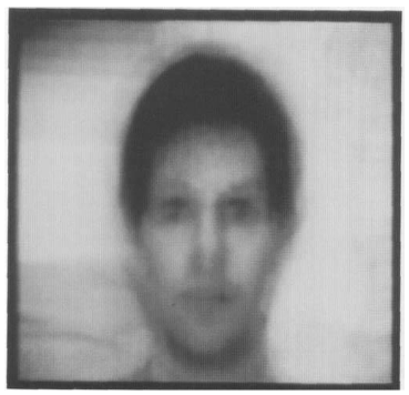
Visualizing Average Face and Eigenfaces
This has all been explained in terms of the maths so far. If we de-vectorize the process, we get the following image for the average face:
and the eigenfaces for each subject:
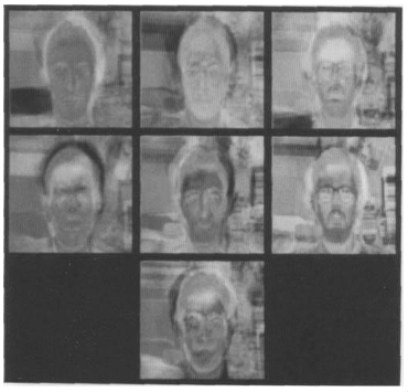
These can be visualized because the average face and the eigenfaces are jsut vectors too.
Reconstructing the Original Image
If we take an image of a face and then create the eigenvectors, etc., then discard the 150 that aren't useful to us, then transform in the face space, then for faces in the database, we get a similar image out.
If the image is not of a face at all, e.g., a flower, we get nothing that looks like a face, but a conglomerate of each different part of the faces that a principal component has tried to extract.
Why Limit the Number of Coefficients
One of the important parts of PCA is to reduce the dimensionality. Take the following image:
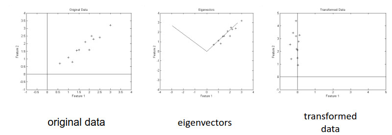
The data is in the format feature 1, feature 2 on the graph. In the 2D space, we'd get the graph on the left but with many more dimensions.
When we do the PCA, we get one important vector, which correlates strongly with the points. The line in the second graph to the left isn't of much use, as the important part of the data is the feature showing strong \(x=y\) correlation.
From this, we have 200 features. Only the top 50 of these features are useful, as the remainder show the vectors similar to \(y = -x\). We select the top 50 from the eigenvalues we get.
SVD
This is similar to PCA, and gives eigenvalues and eigenvectors. It is called single value decomposition.
Recognition vs Verification
The approaches so far have focused on the recognition of a person within the dataset. Verification is the process of ensuring that the image of the person is a true match, instead of recognition, which is just using the nearest person.
For verification, we can set limits on the distance from the dataset in the feature space. If the distance is below some threshold, then we can verify or reject. This gives a binary yes or no as to whether a person can be authenticated as a person in the database.
Results on Changing Parts of the System
The following image shows a graph, with the performance of the system in relation to:
- (a) the lighting
- (b) the head size
- (c) the orientation of the image
- (d) a combination of orientation and lighting
- (e) the orientation and size
- (f) the orientation and size also
- (g) size and lighting
- (h) size and lighting again
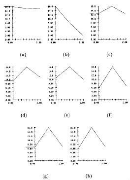
This was examined in Turk and Pentland J. Cog. Neuroo. vol. 3, no. 1, 1991
Recent Algorithms
More modern algorithms use a resnet with a loss function belonging to different faces, but this isn't needed for the exam.
Haar Wavelets
Often, we have a face within an image, and we want to somehow locate the face within the image. We want to have a bounding box around the face. We can use algorithms for this for things such as autofocus, or to classify a face.
The early ways to solve this was to use a Haar wavelet, which is in the Feature Extraction and Image Processing book. Sometimes it is known as the Haar filter. The algorithm used is called a Viola Jones algorithm, from M. Viola, M.J. Jones, IJCV, 2004.
the filter is rectangular, with two black squares on either side, connected at the bottom by a small black line. The middle part corresponds to the nose, and each of the dark parts either side corresponds to the eyes.
Once we locate the eyes, then we can get an estimate for the location of the face(s) in the image. We can use a bank of these filters at different orientations to extract not only the faces that are at the correct orientation, but at different orientations too.
We can then do a correlation of the Haar filters with the image, to see what matches we yield. The best matches will have the highest score of the bank, and then we can find where the face is. This was an early method, and since then, we have newer models based on networks, including YOLO and RCNN, which can detect any object we want, provided the object already exists in the training data.
YOLO was introduced in 2016: Redmon, DIvvala, et. al: CVPR, pp: 779-788, 2016. RCNN was also introduced around the same time, and is constantly evolving.
Face Datasets
There are a few datasets containing faces in literature. One of these is FERET, which contains a database of faces with different facial expressions (happy, sad, neutral, etc.). The dataset contains several images of the same expression from the same subject facing the camera, 90° to the left, 90° to the right, and two further in between centre and sideways.
Further datasets including the Notre Dame HumanID database, where faces are against lots of different backgrounds in differing lighting. There is also the University of Texas video database, which gives example images for different recording conditions.
Recognition under Changing Illumination
Illumination is a key part of good facial recognition. For images that are not preprocessed, the accuracy of a recognition system sharply decreases as the lighting becomes less favourable. This is because less lighting causes more shadow, reducing the accuracy of the algorithm.
With the application of some preprocessing, then we can keep the recognition rate at about 90%. One proposed method by X. Tan and B. triggs, IEEE TIP, 2010 takes a raw image, then normalizes the illumination, before feature extraction, subspace representation and the output.
For the normalization step, we take an input, do a gamma correction, take a difference of Gaussians filter, do some masking, then take an equalization of variation to get the final image.
From doing a histogram equalization, we get the histogram to be a wider range of values than the output from the difference of Gaussians output.
Following all this, we will have done the illumination normalization. From the resultant image, we then need a feature extraction technique to get data for classification.
Gamma Correction
For an image \(V_{in}^\gamma\), with \(\gamma\) a value that changes from e.g., \(1/4,1/3,1/2,1,2\), we can produce an image \(V_{out}\). The higher the \(\gamma\), the darker the image becomes.
For a face that has uneven lighting (e.g., the LHS of the face is well lit, and the RHS is not), then we can correct the gamma on the side that is not well lit by taking an estimate of the gamma on the LHS and applying it to the RHS.
Difference of Gaussians
Warning
This is done on the whiteboard and is not legible from the recordings.
This is similar to difference of Laplacian, being the second derivative of a Gaussian filter with respect to \(x\).
For \(\sigma\) as the standard deviation, we have \(G_{\sigma} - G_{\sigma+\eta \sigma}\), which is the difference of the two?
Difference of Gaussians gives the image, where we make it more intense where there is a change in the lighting.
Local Binary Patterns
This is a feature extraction technique that can be applied to faces, which is normally used for texture classification. We can have a different size for the kernel. For a \(3\times3\) window for images, we apply thresholding on the pixels within to get a binary output:
which gives the binary code \(11000011\). This can be applied to larger kernels, but the binary code for the one demonstrated shows 8-bits.
Once calculated, we move the window one pixel to the right, then calculate the binary code for the next pixel to the right. This then gives a feature map. From here, we can take a histogram of the feature map, to yield information.
Combining Multiple Features
The paper mentioned earlier combines the LBP with Gabor features and other features. They use the kernel classifier in the kernel subspace, noramlize with a Z-score, then fuse the scores together.
The kernel subspace adds the values together for each method tried, then the sum of all these values gives one distance for one face from the training dataset.
Challenges in Facial Recognition
The main issues with facial recognition are the lighting and illumination of the subject, where the camera is (e.g., the angle), occlusions of the face, resolution of the images, the expression on the face, ageing, and make-up or other cosmetics on the skin.
For the viewpoint issue, there is a dataset LFW, which has faces from all angles.
Facial Expression Analysis
Gabor wavelets can come in handy again, as they can extract different subimages from the initial image.
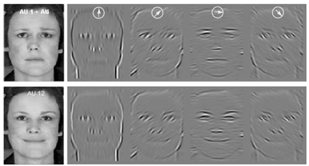
Within the image, the angle of the sine is given at the top. Therefore, for the same person, a different facial expression will yield a different histogram. We need an algorithm which allows us to recognise a face even if the facial expression on the face is different.
Component Facial Expression Analysis
Component facial expression analysis is the process of taking an action face, e.g., one with an expression, and comparing it to the neutral position of the face.
From these, we can calculate difference images as \(\text{difference} = | \text{action face} - \text{neutral face} |\). Once we have this difference, we can then separate the information about the face from the information about the expression of the face.
The difference image is used with PCA or ICA (independent component analysis) in order to analyse the expression and extract features, which can be preserved to describe the expression.
PCA Recap
In PCA, we have an image or vector of an image \(X\) as \(X = \bar{X} + a_1\vec{e}_1 + a_2\vec{e}_2 + \cdots + a_N\vec{e}_N\). We have \(N\) eigenvectors and eigenvalues for \(N\), which is the number of coefficients.
Recall that each eigenvector is orthogonal to the rest:
These are known as 'orthonormal' vectors. They have unit length.
ICA
ICA is similar to PCA, in that we have a feature vector \(X\) for each image.
In this form, the vectors \(\vec{v}_i\) are independent basis functions. They are orthogonal and have unity. These properties are the same as the PCA properties.
The difference with ICA is that instead of taking the eigenvectors and eigenvalues from the covariance matrix in the data, we have constant basis functions that are independently generated and calculated.
The main aim with component facial expression analysis is to be able to quantify what expression a person has based on the analysis of their face. The main paper for this is B. Fasel, J. Luettin, Pattern Recognition, 36, 2003.
Active Shape Models
Similar to the hands which consist of a set of points, active shape models aim to represent a face similarly to the hand, by tracking it as a collection of different points. PCA can be applied in exactly the same way.
These points have an \((x,y)\). By changing the coefficients of the eigenvectors for the faces, we can generate new faces. We can also generate different expressions for the same person. This is known as the active shape model.
Active shape models also allow us to segment the face by fitting the model/template (a set of points comprising the drawn face) and iteratively trying to minimize some term with the algorithm trying to calculate the best match between the drawing and the face. Once the best match has been reached, we are in the minimum of the function.
After segmenting the face, we can then use PCA again to extract features from the face. If we make use of the grayscale skin tones within the main shape, we can then call the model an active appearance model.
Face Ageing (AAM)
AAM (active appearance model) allows us to change the age of a person. Using PCA, we can then de-age a person, using our trained model on the ageing of the face. This was discussed in E. Patterson, A. Sethuram et al;., IEEE BTAS
Age Estimation
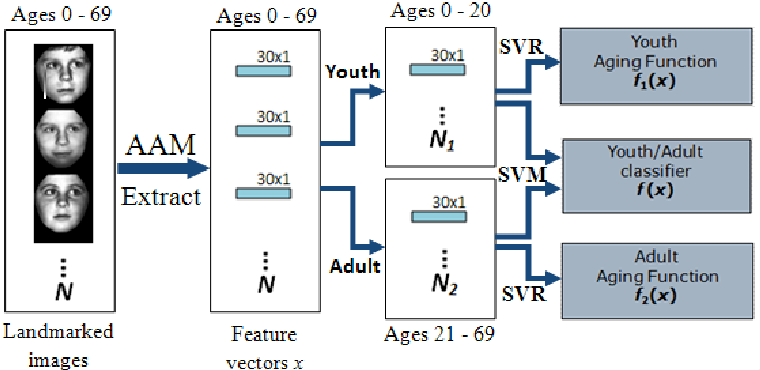
Face ageing has been used to train an age estimation model. We take images with a concrete age, then extract the PCA features with AAM to get a set of \(N\) feature vectors \(N\) with 30 dimensions. We then split the feature vectors for persons 0-20 and then from ages 21-69.
Following this, we can use SVR (support vector regognition) to recognise youth, and ageing adults using the data from the respective splits, then make use of SVM (support vector machines) to classify youth/adults in the middle. This, visually, looks like:
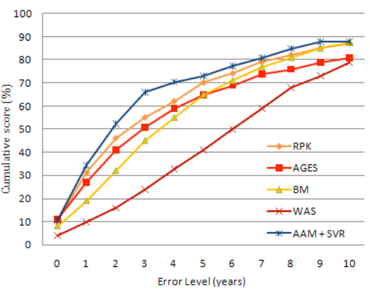
Once the classifiers are trained, we can then use the PCA of a live subject to age a person based on an image. SVM classifies the image as either young or adult, then we use the output of the ageing function that the SVM recommends. The lecture slides also show a CMC plot, showing that the cumulative score of AAM+SVR is higher than other methods.
The CMC plot tracks the cumulative score against the error level we allow (in years).
Future Work
Future work includes the attributes of the faces, the influence of deep neural networks on these recognition techniques, and the use of labelled faces in the wild database.